Log link in Poisson ash
Table of Contents
Introduction
We previously found several instances of genes which clearly exhibit unimodal expression variation (by inspection), but significantly depart from the estimated unimodal distribution
\begin{align*} x_i \mid s_i, \lambda_i &\sim \operatorname{Poisson}(s_i \lambda_i)\\ \lambda_i &\sim g(\cdot) = \sum_{k=1}^K w_k \operatorname{Uniform}(\lambda_0, a_k) \end{align*}where \(\lambda_0\) is the mode and we abuse notation to allow endpoints \(a_k < \lambda_0\). One feature which appears to be common to these examples is estimating the density near zero wrong, such that the smallest randomized quantiles deviate from uniform.
Here, we investigate problems in fitting a unimodal assumption under the log link
\begin{align*} x_i \mid s_i, \lambda_i &\sim \operatorname{Poisson}(s_i \lambda_i)\\ \theta_i = \ln \lambda_i &\sim g(\cdot) = \sum_{k=1}^K w_k \operatorname{Uniform}(\theta_0, a_k) \end{align*}Setup
import numpy as np
import pandas as pd
import rpy2.robjects
import rpy2.robjects.pandas2ri
import scipy.integrate as si
import scipy.special as sp
import scipy.stats as st

rpy2.robjects.pandas2ri.activate()
%matplotlib inline
%config InlineBackend.figure_formats = set(['retina'])
import matplotlib.pyplot as plt
plt.rcParams['figure.facecolor'] = 'w'
plt.rcParams['font.family'] = 'Nimbus Sans'
Derivations
Under the log link, we have
\begin{align*} x_i \mid s_i, \lambda_i &\sim \operatorname{Poisson}(s_i \lambda_i)\\ \theta_i = \ln \lambda_i &\sim \operatorname{Uniform}(a, b) \end{align*}and
\begin{align*} \Pr(x_i = x) &= \frac{1}{b - a} \int_a^b \operatorname{Poisson}(x; \exp(\ln s_i + \theta_i))\,d\theta_i\\ &= \frac{1}{b - a} \int_a^b \frac{(s_i)^x}{\Gamma(x + 1)} \exp(\theta_i)^{x}\exp(-s_i \exp(\theta_i))\,d\theta_i\\ &= \frac{1}{x (b - a)} \int_{\exp(a)}^{\exp(b)} \frac{(s_i)^x}{\Gamma(x)} \lambda_i^{x - 1}\exp(-s_i \lambda_i)\,d\lambda_i\\ &= \frac{1}{x (b - a)} \left( F_\Gamma(\exp(b); x, s_i) - F_\Gamma(\exp(a); x, s_i) \right)\\ \Pr(x_i \leq x) &= \sum_{k=0}^{x} \frac{1}{k (b - a)} \left( F_\Gamma(\exp(b); k, s_i) - F_\Gamma(\exp(a); k, s_i) \right) \end{align*}where \(F_\Gamma(\cdot; \alpha, \beta)\) denotes the CDF of the Gamma distribution with shape \(\alpha\) and rate \(\beta\). This derivation breaks down for \(\Pr(x_i = 0)\), because the Gamma distribution is not defined for \(\alpha = 0\), and because there is a factor of \(1 / x_i\). Instead,
\begin{align*} \Pr(x_i = 0) &= \frac{1}{b - a} \int_{\exp(a)}^{\exp(b)} \frac{\exp(-s_i \lambda_i)}{\lambda_i}\,d\lambda_i\\ &= \frac{1}{b - a} \int_{-s_i \exp(a)}^{-s_i \exp(b)} \frac{\exp(t)}{t}\,dt\\ &= \frac{\operatorname{Ei}(-s_i \exp(b)) - \operatorname{Ei}(-s_i \exp(a))}{b - a} \end{align*}where \(\operatorname{Ei}\) is the exponential integral.
Compare the estimate of \(\ln \Pr(x_i = 0 \mid x_i+)\) using numerical integration, the special case analytic formula involving \(\operatorname{Ei}\), and introducing a pseudocount into the formula involving \(F_\Gamma\).
# Typical values
s = np.logspace(0, 6, 20)
a = np.log(2e-3)
b = np.log(3e-3)

# Numerical integration
px_0 = np.array([si.quad(lambda x: st.poisson(mu=s_j * np.exp(x)).pmf(0), a, b)[0] / (b - a) for s_j in s])

# Analytic
px_1 = (sp.expi(-s * np.exp(b)) - sp.expi(-s * np.exp(a))) / (b - a)

# Follow ashr
eps = 1e-5
F = st.gamma(a=eps, scale=1 / s).cdf
px_2 = (F(np.exp(b)) - F(np.exp(a))) / (eps * (b - a))

np.log(pd.DataFrame({'quad': px_0, 'Ei': px_1, 'F_gamma': px_2}, index=s))
quad          Ei    F_gamma
1.000000         -0.002466   -0.002466  -0.002521
2.069138         -0.005103   -0.005103  -0.005150
4.281332         -0.010558   -0.010558  -0.010598
8.858668         -0.021845   -0.021845  -0.021877
18.329807        -0.045193   -0.045193  -0.045218
37.926902        -0.093480   -0.093480  -0.093498
78.475997        -0.193290   -0.193290  -0.193301
162.377674       -0.399380   -0.399380  -0.399383
335.981829       -0.823968   -0.823968  -0.823964
695.192796       -1.694739   -1.694739  -1.694728
1438.449888      -3.464673   -3.464673  -3.464655
2976.351442      -7.008214   -7.008214  -7.008189
6158.482111     -13.999734  -13.999734 -13.999714
12742.749857    -27.858046  -27.858046       -inf
26366.508987    -55.813991  -55.813991       -inf
54555.947812   -112.910591 -112.910591       -inf
112883.789168  -230.288764 -230.288764       -inf
233572.146909  -472.390342 -472.390345       -inf
483293.023857         -inf        -inf       -inf
1000000.000000        -inf        -inf       -inf
Matthew Stephens provided an alternative derivation:
\begin{align*} \Pr(x_i = x) &= \frac{1}{b - a} \int_a^b \operatorname{Poisson}(x; \exp(\ln s_i + \theta_i))\,d\theta_i\\ &= \frac{1}{b - a} \int_{\exp(a)}^{\exp(b)} \frac{s_i^x}{\Gamma(x + 1)} \lambda_i^{x - 1}\exp(-s_i \lambda_i)\,d\lambda_i\\ &= \frac{1}{\Gamma(x + 1) (b - a)} \int_{s_i \exp(a)}^{s_i \exp(b)} u^{x-1} \exp(-u)\,du\\ &= \frac{1}{\Gamma(x + 1) (b - a)} \left( \Gamma(x, s_i \exp(a)) - \Gamma(x, s_i \exp(b)) \right) \end{align*}where \(\Gamma(\cdot, \cdot)\) is the upper incomplete Gamma function. The resulting expression is defined for all \(x \geq 0\).
Results
Simulated data
Simulate some near-NB ZINB data.
dat <- readRDS("/scratch/midway2/aksarkar/modes/test-data/pois-mode-est.Rds")
with(dat, summary(MASS::glm.nb(x ~ offset(log(s))))$twologlik / 2)
-2008.50373054974
Fit ash_pois using identity link.
fit0 <- ashr::ash_pois(dat$x, dat$s, link="identity", mixcompdist="halfuniform")
fit0$loglik
-2008.27125771255
Implement
autoselect.mixsd for log link.
Fit ash_pois using log link. (The problem turned out to be
mode
estimation limits.)
fit1 <- ashr::ash_pois(dat$x, dat$s, link="log", mixcompdist="halfuniform")
fit1$loglik
-2008.26590367036
Real data
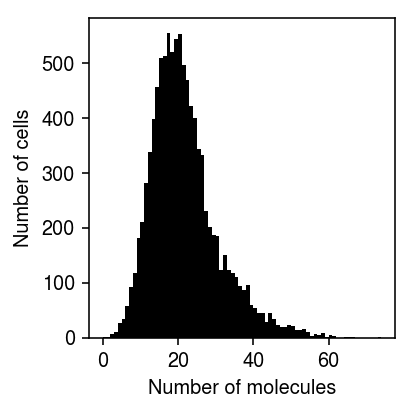
Load a real data example which is clearly unimodal, but departs from the fitted distribution.
dat <- readRDS("/scratch/midway2/aksarkar/modes/test-data/b-cell-data.Rds")
query <- dat[dat["gene"] == "ENSG00000019582",]
data = pd.DataFrame(rpy2.robjects.r['readRDS']("/scratch/midway2/aksarkar/modes/test-data/b-cell-data.Rds"))
query = data[data["gene"] == "ENSG00000019582"]
Plot the empirical distribution of molecule counts.
plt.clf()
plt.gcf().set_size_inches(3, 3)
plt.hist(query['count'], bins=np.arange(query['count'].max() + 1), color='k')
plt.xlabel('Number of molecules')
plt.ylabel('Number of cells')
plt.tight_layout()
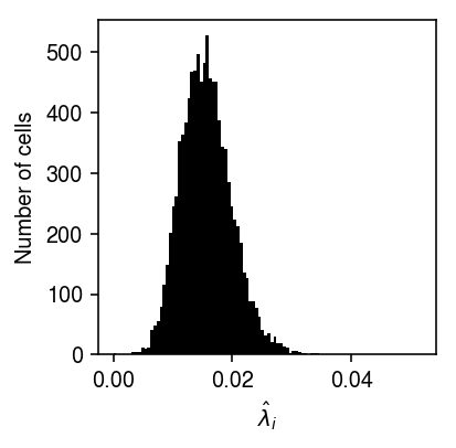
Plot the distribution of MLEs \(x_i / s_i\).
plt.clf()
plt.gcf().set_size_inches(3, 3)
plt.hist(query['count'] / query['size'], bins=100, color='k')
plt.xlabel('$\hat\lambda_i$')
plt.ylabel('Number of cells')
plt.tight_layout()
As a baseline, fit a Gamma assumption.
with(query, summary(MASS::glm.nb(count ~ offset(log(size))))$twologlik / 2)
-31414.5999341206
Fit a unimodal assumption under the identity link.
fit0 <- ashr::ash_pois(query$count, query$size, link="identity", mixcompdist="halfuniform")
fit0$loglik
-31395.0538031464
Report the diagnostic test statistic and p-value.
zgrep -wm1 ENSG00000019582 /project2/mstephens/aksarkar/projects/singlecell-modes/data/gof/b_cells-unimodal.txt.gz
Fit a unimodal assumption under the log link.
fit1 <- ashr::ash_pois(query$count, query$size, link="log", mixcompdist="halfuniform")
fit1$loglik
-31394.8462180293
Make sure the marginal PMF is sensible. (This was not implemented correctly before.)
any(fit1$fitted_g$pi %*% ashr:::comp_dens_conv(fit1$fitted_g, fit1$data) > 1)
FALSE
any(ashr:::comp_dens_conv(fit1$fitted_g, fit1$data) > 1)
FALSE
Implement the diagnostic for the log link.
fx = fit1$fitted_g$pi %*% ashr:::comp_dens_conv(fit1$fitted_g, fit1$data)
N = nrow(query)
K = length(fit1$fitted_g$a)
## Important: this is F_j(x_{ij} - 1), needed for randomized quantiles
Fx_1 = matrix(rep(0, N * K), N, K)
for (i in 1:N) {
  for (k in 1:K) {
    if (fit1$fitted_g$pi[k] < 1e-8) {
      next
    }
    else if (query$count[i] == 0) {
      Fx_1[i, k] = 0
    }
    else if (fit1$fitted_g$a[k] == fit1$fitted_g$b[k]) {
      Fx_1[i, k] = ppois(query$count[i] - 1, lambda=query$size[i] * exp(fit1$fitted_g$a[k]))
    }
    else {
      ak = min(fit1$fitted_g$a[k], fit1$fitted_g$b[k])
      bk = max(fit1$fitted_g$a[k], fit1$fitted_g$b[k])
      grid = seq(0, query$count[i] - 1)
      Fx_1[i, k] = sum((expint::gammainc(grid, query$size[i] * exp(ak)) -
                          expint::gammainc(grid, query$size[i] * exp(bk))) /
                         (gamma(grid + 1) * (bk - ak)))
    }
  }
}
rpp = drop(Fx_1 %*% fit1$fitted_g$pi) + runif(n=N) * fx
ks.test(rpp, punif)$p.value
0.00683832270839435