Goodness of fit of deconvolved distributions
Table of Contents
Introduction
We previously estimated the out-of-sample log likelihood as a measure of the generalization performance of distribution deconvolution methods for scRNA-seq. However, this is not the simplest way to support our key results:
- For control experiments, the data do not significantly depart from a unimodal distribution for expression variation (meaning, neither sequencing variation nor expression variation involve a point mass on zero).
- For most genes, in most data sets, the data do not significantly depart from a Gamma assumption.
- When the data do significantly depart from a Gamma assumption, they often do not depart from a unimodal assumption (meaning, departures from Gamma are often not due to excess zeros).
Here, we directly test for the goodness of fit of the estimated distributions (as in Sarkar et al. 2019).
Setup
import anndata
import numpy as np
import pandas as pd
import scanpy as sc
import scmodes
import colorcet
import os
import rpy2.robjects
import rpy2.robjects.packages
import scipy.io as si
import scipy.special as sp
import scipy.stats as st
import scqtl
import sqlite3

ashr = rpy2.robjects.packages.importr('ashr')
%matplotlib inline
%config InlineBackend.figure_formats = set(['retina'])
import matplotlib.pyplot as plt
plt.rcParams['figure.facecolor'] = 'w'
plt.rcParams['font.family'] = 'Nimbus Sans'
Methods
Test for goodness of fit
The key idea underlying our test for goodness of fit is the fact that if \(x_{i} \sim F(\cdot)\), then \(F(x_{i}) \sim \operatorname{Uniform}(0, 1)\). To test for goodness of fit of an estimated \(\hat{F}\) to the data \(x_{1}, \ldots, x_{n}\), we apply the Kolmogorov-Smirnov (KS) test to test whether the values \(\hat{F}(x_1), \ldots, \hat{F}(x_n)\) are uniformly distributed. (This test is slightly conservative because it uses the same data to estimate \(\hat{F}\).)
Here, we have to modify this simple procedure to account for the fact that our data are discrete counts, so \(F\) is not continuous. To address this issue, we used randomized quantiles (Dunn 1996): we sample one random value per observation \(u_{i} \mid x_{i} \sim \mathrm{Uniform}(\hat{F}(x_i - 1), \hat{F}(x_i))\). These have the property that if \(x_i \sim F\) then \(u_i \sim \mathrm{Uniform}(0, 1)\).
In our model, each observed UMI count \(x_{i}\) comes from a different distribution \(F_{i}\):
\[ F_i(x_i) = \sum_{k=0}^{x_i} \int_0^\infty \operatorname{Poisson}(k; x_i^+ \lambda_i) g(d\lambda_i) \]
We therefore draw \(u_{i} \mid x_{i} \sim \mathrm{Uniform}(\hat{F}_{i}(x_{i} - 1), \hat{F}_{i}(x_{i}))\). Then, we apply the KS test to whether the randomized quantiles \(u_{i}\) are uniformly distributed.
Poisson-unimodal goodness of fit
We parameterized the Poisson-unimodal model as:
\begin{align*} x_i &\sim \operatorname{Poisson}(x_i^+ \lambda_i)\\ \lambda_i &\sim \sum_k w_k \operatorname{Uniform}(\lambda_0, a_k) \end{align*}where we abuse notation to allow \(a_k < \lambda_0\). To test for goodness of fit, we need the PMF and CDF of \(x_i\), marginalized over \(\lambda_i\). These are analytic for certain choices of likelihood and prior, e.g. normal likelihood and mixture of uniforms prior.
Simulate a continuous example.
bhat = pd.Series(np.random.normal(loc=0.1, size=1000))
fitn = ashr.ash_workhorse(bhat, 1, mixcompdist='uniform', output=pd.Series(['loglik', 'fitted_g', 'data']))
# Important: Normal-uniform convolution CDF is analytic
F = np.array(fitn.rx2('fitted_g').rx2('pi')).dot(np.array(ashr.comp_cdf_conv(fitn.rx2('fitted_g'), fitn.rx2('data'))))
st.kstest(F, 'uniform')
KstestResult(statistic=0.03101662170773789, pvalue=0.28605255994768175)
For the Poisson-unimodal model, we have (for one component):
\begin{align*} x_i &\sim \operatorname{Poisson}(x_i^+ \lambda_i)\\ \lambda_i &\sim \operatorname{Uniform}(a, b) \end{align*}and:
\begin{align*} \Pr(x_i = x) &= \int_0^\infty \operatorname{Poisson}(x; x_i^+ \lambda_i) \operatorname{Uniform}(a, b)\,d\lambda_i\\ &= \frac{1}{b - a} \int_a^b \operatorname{Poisson}(x; x_i^+ \lambda_i)\,d\lambda_i\\ &= \frac{1}{x_i^+ (b - a)} \int_a^b \frac{(x_i^+)^{x + 1}}{\Gamma(x + 1)} \lambda_i^{(x + 1) - 1}\exp(-x_i^+ \lambda_i)\,d\lambda_i\\ &= \frac{1}{x_i^+ (b - a)} \left( F_\Gamma(b; x + 1, x_i^+) - F_\Gamma(a; x + 1, x_i^+) \right)\\ \Pr(x_i \leq x) &= \sum_{k=0}^{x} \frac{1}{x_i^+ (b - a)} \left( F_\Gamma(b; k + 1, x_i^+) - F_\Gamma(a; k + 1, x_i^+) \right) \end{align*}where \(F_\Gamma(\cdot; \alpha, \beta)\) denotes the CDF of the Gamma distribution with shape \(\alpha\) and rate \(\beta\). The marginal PMF is analytic. Computing the CDF for each data point, for each component gives a matrix of values \(\mathbf{F} = [F_{ik}]\). Then, the marginal CDF of the data is given by \(\mathbf{F}\mathbf{w}\).
Simulate a simple discrete example.
y = pd.Series(np.random.poisson(lam=10, size=1000))
s = pd.Series(np.ones(y.shape))
fitp = ashr.ash_workhorse(
  np.zeros(y.shape), 1,
  lik=ashr.lik_pois(y=y, scale=s, link='identity'),
  mixcompdist='halfuniform',
  output=pd.Series(['loglik', 'fitted_g', 'data']))
scmodes.benchmark.gof._gof(y,
  cdf=scmodes.benchmark.gof._ash_cdf,
  pmf=scmodes.benchmark.gof._ash_pmf, fit=fitp, s=s)
KstestResult(statistic=0.018791616085501672, pvalue=0.8718125394494075)
Simulate a Poisson example with varying size factors.
mu = 1e-3
s = pd.Series(np.random.poisson(lam=1000, size=10000))
y = pd.Series(np.random.poisson(lam=s * mu))
fitp = ashr.ash_workhorse(
  np.zeros(y.shape), 1,
  lik=ashr.lik_pois(y=y, scale=s, link='identity'),
  mixcompdist='halfuniform',
  output=pd.Series(['loglik', 'fitted_g', 'data']))
scmodes.benchmark.gof._gof(y,
  cdf=scmodes.benchmark.gof._ash_cdf,
  pmf=scmodes.benchmark.gof._ash_pmf, fit=fitp, s=s)
KstestResult(statistic=0.008062709224521236, pvalue=0.533974089244596)
An alternative parameterization is to assume the log link. For one component,
\begin{align*} x_i &\sim \operatorname{Poisson}(x_i^+ \lambda_i)\\ \theta_i = \ln \lambda_i &\sim \operatorname{Uniform}(a, b) \end{align*}and
\begin{align*} \Pr(x_i = x) &= \frac{1}{b - a} \int_a^b \operatorname{Poisson}(x; \exp(\ln x_i^+ + \theta_i))\,d\theta_i\\ &= \frac{1}{b - a} \int_a^b \frac{(x_i^+)^x}{\Gamma(x + 1)} \exp(\theta_i)^{x}\exp(-x_i^+ \exp(\theta_i))\,d\theta_i\\ &= \frac{1}{x (b - a)} \int_{\exp(a)}^{\exp(b)} \frac{(x_i^+)^x}{\Gamma(x)} \lambda_i^{x - 1}\exp(-x_i^+ \lambda_i)\,d\lambda_i\\ &= \frac{1}{x (b - a)} \left( F_\Gamma(\exp(b); x, x_i^+) - F_\Gamma(\exp(a); x, x_i^+) \right)\\ \Pr(x_i \leq x) &= \sum_{k=0}^{x} \frac{1}{k (b - a)} \left( F_\Gamma(\exp(b); k, x_i^+) - F_\Gamma(\exp(a); k, x_i^+) \right) \end{align*}Data
def read_chromium(sample):
  x = sc.read('/project2/mstephens/aksarkar/projects/singlecell-modes/data/negative-controls/svensson_chromium_control.h5ad')
  x = x[x.obs['sample'] == sample]
  sc.pp.filter_genes(x, min_cells=1)
  x = x[:,x.var.filter(like='ERCC', axis='index').index]
  return pd.DataFrame(x.X.A, index=x.obs.index, columns=x.var.index)

def read_dropseq():
  x = sc.read('/project2/mstephens/aksarkar/projects/singlecell-modes/data/negative-controls/macosko_dropseq_control.h5ad')
  sc.pp.filter_genes(x, min_cells=1)
  x = x[:,x.var.filter(like='ERCC', axis='index').index]
  return pd.DataFrame(x.X.A, index=x.obs.index, columns=x.var.index)

def read_indrops():
  x = sc.read('/project2/mstephens/aksarkar/projects/singlecell-modes/data/negative-controls/klein_indrops_control.h5ad')
  sc.pp.filter_genes(x, min_cells=1)
  x = x[:,x.var.filter(like='ERCC', axis='index').index]
  return pd.DataFrame(x.X.A, index=x.obs.index, columns=x.var.index)

def read_gemcode():
  x = sc.read('/project2/mstephens/aksarkar/projects/singlecell-modes/data/negative-controls/zheng_gemcode_control.h5ad')
  sc.pp.filter_genes(x, min_cells=1)
  return pd.DataFrame(x.X.A, index=x.obs.index, columns=x.var.index)

def _mix_10x(k1, k2, min_detect=0.01, return_y=False):
  x1 = scmodes.dataset.read_10x(f'/project2/mstephens/aksarkar/projects/singlecell-ideas/data/10xgenomics/{k1}/filtered_matrices_mex/hg19/', return_df=True, min_detect=0)
  x2 = scmodes.dataset.read_10x(f'/project2/mstephens/aksarkar/projects/singlecell-ideas/data/10xgenomics/{k2}/filtered_matrices_mex/hg19/', return_df=True, min_detect=0)
  x, y = scmodes.dataset.synthetic_mix(x1, x2, min_detect=min_detect)
  if return_y:
    return x, y
  else:
    return x

def _cd8_cd19_mix(**kwargs):
  return _mix_10x('cytotoxic_t', 'b_cells', **kwargs)

def _cyto_naive_mix(**kwargs):
  return _mix_10x('cytotoxic_t', 'naive_t', **kwargs)

def _read_10x(k, return_df=True, min_detect=0.01):
  return scmodes.dataset.read_10x(f'/project2/mstephens/aksarkar/projects/singlecell-ideas/data/10xgenomics/{k}/filtered_matrices_mex/hg19/',
                                  return_adata=not return_df, return_df=return_df, min_detect=min_detect)

def read_liver():
  x = anndata.read_h5ad('/project2/mstephens/aksarkar/projects/singlecell-ideas/data/human-cell-atlas/liver-caudate-lobe/liver-caudate-lobe.h5ad')
  sc.pp.filter_genes(x, min_cells=.01 * x.shape[0])
  return x

def read_kidney():
  x = anndata.read_h5ad('/project2/mstephens/aksarkar/projects/singlecell-ideas/data/human-cell-atlas/kidney/kidney.h5ad')
  sc.pp.filter_genes(x, min_cells=.01 * x.shape[0])
  return x

def read_brain():
  x = anndata.read_h5ad('/project2/mstephens/aksarkar/projects/singlecell-ideas/data/gtex-droncseq/gtex-droncseq.h5ad')
  sc.pp.filter_genes(x, min_counts=.01 * x.shape[0])
  return x

def read_retina():
  x = anndata.read_h5ad('/project2/mstephens/aksarkar/projects/singlecell-ideas/data/human-cell-atlas/adult-retina/adult-retina.h5ad')
  query = x.obs['donor_organism.provenance.document_id'] == '427c0a62-9baf-42ab-a3a3-f48d10544280'
  y = x[query]
  sc.pp.filter_genes(y, min_cells=.01 * y.shape[0])
  return y

data = {
  'dropseq': read_dropseq,
  'indrops': read_indrops,
  'chromium1': lambda: read_chromium('20311'),
  'chromium2': lambda: read_chromium('20312'),
  'gemcode': read_gemcode,
  'cytotoxic_t': lambda: _read_10x('cytotoxic_t'),
  'b_cells': lambda: _read_10x('b_cells'),
  'ipsc': lambda: scmodes.dataset.ipsc('/project2/mstephens/aksarkar/projects/singlecell-qtl/data/', return_df=True),
  'cytotoxic_t-b_cells': _cd8_cd19_mix,
  'cytotoxic_t-naive_t': _cyto_naive_mix,
  'pbmcs_68k': lambda: _read_10x('fresh_68k_pbmc_donor_a', return_df=False),
  'liver-caudate-lobe': read_liver,
  'kidney': read_kidney,
  'brain': read_brain,
  'retina': read_retina,
}
Report the dimensions of each data set.
pd.DataFrame([data[k]().shape for k in data],
             columns=['num_cells', 'num_genes'],
             index=data.keys())
num_cells  num_genes
dropseq                     84         81
indrops                    953        103
chromium1                 2000         88
chromium2                 2000         88
gemcode                   1015         91
cytotoxic_t              10209       6530
b_cells                  10085       6417
ipsc                      5597       9957
cytotoxic_t-b_cells      20294       6647
cytotoxic_t-naive_t      20688       6246
pbmcs_68k                68579       6502
liver-caudate-lobe        8856       3181
kidney                   11233      15496
brain                    14963      11744
retina                   21285      10047
Results
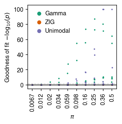
Simulation
Draw data following the Poisson-point Gamma distribution:
\begin{align*} x_i &\sim \operatorname{Poisson}(x_i^+ \lambda_i)\\ \lambda_i &\sim \pi \delta_0(\cdot) + (1 - \pi) \operatorname{Gamma}(1/\phi, 1/(\mu\phi)) \end{align*}Draw simulation parameters \(x_i^+=10^5, \ln\mu, \ln\phi\) from typical values (Sarkar et al. 2019).
\begin{align*} \ln\mu &\sim \operatorname{Uniform}(-12, -8)\\ \ln\phi &\sim \operatorname{Uniform}(-6, 0) \end{align*}Then, test for goodness of fit of Gamma, point-Gamma, and unimodal, each convolved with Poisson.
import scmodes.benchmark.gof

def trial(num_samples, logodds, seed, verbose=False):
  data, _ = scqtl.simulation.simulate(num_samples=num_samples, logodds=logodds, seed=seed)
  x = data[:,0]
  s = data[:,1]
  # Important: scqtl.simple returns mu, 1/phi
  fit0 = scqtl.simple.fit_nb(x, s)
  res0 = scmodes.benchmark.gof._gof(x, cdf=scmodes.benchmark.gof._zig_cdf,
                                    pmf=scmodes.benchmark.gof._zig_pmf, size=s,
                                    log_mu=np.log(fit0[0]), log_phi=-np.log(fit0[1]))
  fit1 = scqtl.simple.fit_zinb(x, s)
  res1 = scmodes.benchmark.gof._gof(x, cdf=scmodes.benchmark.gof._zig_cdf,
                                    pmf=scmodes.benchmark.gof._zig_pmf, size=s,
                                    log_mu=np.log(fit1[0]), log_phi=-np.log(fit1[1]), logodds=fit1[2])

  # Important: this returns the gene name as the first return value
  res2 = scmodes.benchmark.gof._gof_unimodal('gene', pd.Series(x), pd.Series(s))
  return res0[1], res1[1], res2[2]

def evaluate(num_samples, num_trials):
  result = []
  for logodds in np.linspace(-5, 0, 10):
    for seed in range(num_trials):
      gamma_res, zig_res, unimodal_res = trial(num_samples, logodds, seed)
      result.append([logodds, seed, gamma_res, zig_res, unimodal_res])
  result = pd.DataFrame(result)
  result.columns = ['logodds', 'trial', 'gamma', 'zig', 'unimodal']
  return result
Run the simulation.
sim_res = evaluate(num_samples=1000, num_trials=10)
Write out the results.
sim_res.to_csv('/project2/mstephens/aksarkar/projects/singlecell-modes/data/gof/simulation.txt.gz', sep='\t', compression='gzip')
Read the results.
sim_res = pd.read_csv('/project2/mstephens/aksarkar/projects/singlecell-modes/data/gof/simulation.txt.gz', sep='\t', compression='gzip', index_col=0)
Plot the results.
cm = plt.get_cmap('Dark2')
plt.clf()
plt.gcf().set_size_inches(3, 3)
for i, (k, l) in enumerate(zip(['gamma', 'zig', 'unimodal'], ['Gamma', 'ZIG', 'Unimodal'])):
  jitter = np.random.normal(scale=0.01, size=sim_res.shape[0])
  plt.scatter(sim_res['logodds'] + jitter, -np.log10(sim_res[k] + 1e-100), s=2, c=np.atleast_2d(cm(i)), label=l)
plt.axhline(y=0, c='k', lw=1)
plt.axhline(y=-np.log10(.05), c='0.8', ls='--', lw=1)
plt.legend(frameon=False, handletextpad=0, markerscale=4)
plt.xticks(np.linspace(-5, 0, 10), [f'{x:.2g}' for x in sp.expit(np.linspace(-5, 0, 10))], rotation=90)
plt.xlabel('$\pi$')
plt.ylabel('Goodness of fit $-\log_{10}(p)$')
plt.tight_layout()
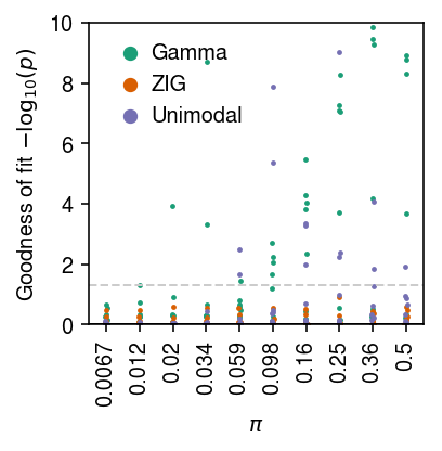
Plot a zoomed-in version of the results.
cm = plt.get_cmap('Dark2')
plt.clf()
plt.gcf().set_size_inches(3, 3)
for i, (k, l) in enumerate(zip(['gamma', 'zig', 'unimodal'], ['Gamma', 'ZIG', 'Unimodal'])):
  jitter = np.random.normal(scale=0.01, size=sim_res.shape[0])
  plt.scatter(sim_res['logodds'] + jitter, -np.log10(sim_res[k] + 1e-100), s=2, c=np.atleast_2d(cm(i)), label=l)
plt.axhline(y=0, c='k', lw=1)
plt.axhline(y=-np.log10(.05), c='0.8', ls='--', lw=1)
plt.legend(frameon=False, handletextpad=0, markerscale=4)
plt.xticks(np.linspace(-5, 0, 10), [f'{x:.2g}' for x in sp.expit(np.linspace(-5, 0, 10))], rotation=90)
plt.xlabel('$\pi$')
plt.ylim(0, 10)
plt.ylabel('Goodness of fit $-\log_{10}(p)$')
plt.tight_layout()
Test for goodness of fit
Run the GPU-based methods.
sbatch --partition=gpu2 --gres=gpu:1 --mem=16G --job-name=gof --time=1:00:00 -a 7
#!/bin/bash
source activate scmodes
python <<EOF
<<imports>>
import os
<<data>>
tasks = list(data.keys())
task = tasks[int(os.environ['SLURM_ARRAY_TASK_ID'])]
x = data[task]()
res = scmodes.benchmark.evaluate_gof(x, methods=['gamma', 'zig'])
res.to_csv(f'/scratch/midway2/aksarkar/modes/gof/{task}-gpu.txt.gz', compression='gzip', sep='\t')
EOF
Move the results to permanent storage.
rsync -au /scratch/midway2/aksarkar/modes/gof/ /project2/mstephens/aksarkar/projects/singlecell-modes/data/gof/
Read the results.
gof_res = []
for m in ['point', 'gpu', 'unimodal', 'npmle']:
  res = dict()
  for k in data:
    f = f'/project2/mstephens/aksarkar/projects/singlecell-modes/data/gof/{k}-{m}.txt.gz'
    if os.path.exists(f):
      # Hacks
      res[k] = pd.read_csv(f, sep='\t', index_col=0)
      if 'ID' in res[k].columns:
        res[k] = res[k].rename({'ID': 'gene'}, axis=1)
      if res[k].index.name == 'ID':
        del res[k]['gene']
        res[k].index.name = 'gene'
      if 'gene.1' in res[k].columns:
        del res[k]['gene.1']
      if m in ('unimodal', 'npmle'):
        res[k] = res[k].reset_index(drop=(res[k].index.name != 'gene'))
  gof_res.append(pd.concat(res, sort=True)
                 .reset_index(level=0)
                 .rename({'level_0': 'dataset'}, axis=1))
gof_res = pd.concat(gof_res).reset_index(drop=True)
Write out the post-processed results.
gof_res.to_csv('/project2/mstephens/aksarkar/projects/singlecell-modes/data/gof/gof.txt.gz', sep='\t', compression='gzip')
Read the post-processed results.
gof_res = pd.read_csv('/project2/mstephens/aksarkar/projects/singlecell-modes/data/gof/gof.txt.gz', sep='\t', index_col=0)
To reduce computational burden, run ashr only on genes which
significantly departed from a Gamma assumption on expression variation in
each dataset. There are several reasons why a gene might depart from the
fitted Gamma expression model:
- The variance is larger than predicted by a Gamma
- The proportion of zeros is larger than predicted by a Gamma
- The true gene expression is multi-modal
- The true gene expression is not independent of the size factor.
Under (2), a point-Gamma model will fit better. Under (3), a unimodal model will not fit the data. Under (4), even a fully non-parametric model will not fit the data.
sig = (gof_res[gof_res['method'] == 'gamma']
       .groupby('dataset')
       .apply(lambda x: x.loc[x['p'] < 0.05 / x.shape[0]]))
for k in data:
  x = data[k]()
  if not isinstance(x, anndata.AnnData):
    if k in sig.index:
      s = x.sum(axis=1)
      # Important: we need to keep around the size factors computed using all the
      # genes
      t = anndata.AnnData(x.loc[:,sig.loc[k, 'gene']].values, var=sig.loc[k, 'gene'].to_frame().set_index('gene'))
      t.obs = s.to_frame().rename({0: 'size'}, axis=1)
      t.write(f'/scratch/midway2/aksarkar/modes/unimodal-data/{k}.h5ad')
  else:
    s = x.X.tocsc().sum(axis=1).A.ravel()
    x.obs['size'] = s
    x.obs = x.obs.rename({0: 'barcode'}, axis=1)
    if x.var.shape[1] == 2:
      x.var.columns = ['gene', 'name']
    else:
      x.var = x.var.rename({'featurekey': 'gene', 'featurename': 'name'}, axis=1)
    x.var = x.var.set_index('gene')
    x[:,x.var.index.isin(sig.loc[k, 'gene'])].write(f'/scratch/midway2/aksarkar/modes/unimodal-data/{k}.h5ad')
sbatch --partition=broadwl -n1 -c28 --exclusive --job-name=gof --time=12:00:00 -a 11-12,26-27
#!/bin/bash
source activate scmodes
python <<EOF
<<imports>>
import anndata
import multiprocessing as mp
import os
import scipy.sparse as ss
<<data>>
tasks = [(m, d) for m in ('unimodal', 'npmle') for d in data]
m, d = tasks[int(os.environ['SLURM_ARRAY_TASK_ID'])]
with mp.Pool(maxtasksperchild=20) as pool:
  # Important: this needs to be done after initializing the pool to avoid
  # memory duplication
  x = anndata.read_h5ad(f'/scratch/midway2/aksarkar/modes/unimodal-data/{d}.h5ad')
  if ss.isspmatrix(x.X):
    y = x.X.A
  else:
    y = x.X
  res = scmodes.benchmark.evaluate_gof(pd.DataFrame(y, index=x.obs.index, columns=x.var.index),
                                       s=x.obs['size'],
                                       pool=pool,
                                       methods=[m])
  res.index = x.var.index
  res.to_csv(f'/scratch/midway2/aksarkar/modes/gof/{d}-{m}.txt.gz', compression='gzip', sep='\t')
EOF
Run goodness of fit tests for a point mass assumption on control data sets only.
sbatch --partition=broadwl --mem=4G --job-name=gof --time=1:00:00 -a 0-4
#!/bin/bash
source activate scmodes
python <<EOF
<<imports>>
import os
<<data>>
tasks = list(data.keys())
task = tasks[int(os.environ['SLURM_ARRAY_TASK_ID'])]
x = data[task]()
res = scmodes.benchmark.evaluate_gof(x, methods=['point'])
res.to_csv(f'/scratch/midway2/aksarkar/modes/gof/{task}-point.txt.gz', compression='gzip', sep='\t')
EOF
Evaluate the log likelihood ratio between the unimodal and non-parametric expression models.
sbatch --partition=broadwl -n1 -c28 --exclusive --job-name=llr --time=12:00:00 -a 6-14
#!/bin/bash
source activate scmodes
python <<EOF
<<imports>>
import anndata
import multiprocessing as mp
import os
import scipy.sparse as ss
<<data>>
tasks = list(data.keys())
d = tasks[int(os.environ['SLURM_ARRAY_TASK_ID'])]
with mp.Pool(maxtasksperchild=20) as pool:
  # Important: this needs to be done after initializing the pool to avoid
  # memory duplication
  x = anndata.read_h5ad(f'/scratch/midway2/aksarkar/modes/unimodal-data/{d}.h5ad')
  if ss.isspmatrix(x.X):
    y = x.X.A
  else:
    y = x.X
  res = scmodes.benchmark.evaluate_lr(pd.DataFrame(y, index=x.obs.index, columns=x.var.index),
                                      s=x.obs['size'],
                                      pool=pool)
  res.index = x.var.index
  res.to_csv(f'/scratch/midway2/aksarkar/modes/gof/{d}-llr.txt.gz', compression='gzip', sep='\t')
EOF
Application to control data sets
Report the number of genes which depart from the null that the data for the gene follows the fitted distribution (after Bonferroni correction at level 0.05).
control = list(data.keys())[:5]
(gof_res[gof_res['dataset'].isin(control)]
 .groupby(['dataset', 'method'])
 .apply(lambda x: (x['p'] < 0.05 / x.shape[0]).sum())
 .reset_index()
 .pivot(index='dataset', columns='method'))
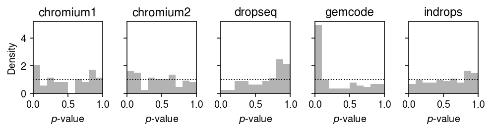
0
method    gamma point unimodal zig
dataset
chromium1     7     9        0   7
chromium2     6    14        0   6
dropseq       0    65        0   0
gemcode      22    28        0  22
indrops       0     2        0   0
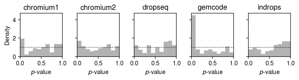
Plot the histogram of goodness of fit test \(p\)-values for the fitted Gamma distributions for each control dataset.
plt.clf()
fig, ax = plt.subplots(1, 5, sharey=True)
fig.set_size_inches(7, 2)
for a, (k, g) in zip(ax.ravel(),
                     gof_res.loc[gof_res['dataset'].isin(control)].groupby('dataset')):
  a.hist(g.loc[g['method'] == 'gamma', 'p'], bins=np.linspace(0, 1, 11), color='0.7', density=True)
  a.axhline(y=1, c='k', ls=':', lw=1)
  a.set_xlim([0, 1])
  a.set_title(k)
ax[0].set_ylabel('Density')
for a in ax:
  a.set_xlabel('$p$-value')
fig.tight_layout()
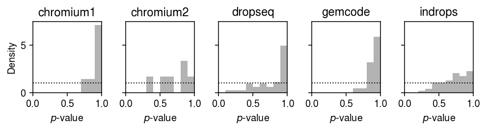
Plot the histogram of goodness of fit test \(p\)-values for the fitted point-Gamma distributions for each control dataset.
plt.clf()
fig, ax = plt.subplots(1, 5, sharey=True)
fig.set_size_inches(7, 2)
for a, (k, g) in zip(ax.ravel(),
                     gof_res.loc[gof_res['dataset'].isin(control)].groupby('dataset')):
  a.hist(g.loc[g['method'] == 'zig', 'p'], bins=np.linspace(0, 1, 11), color='0.7', density=True)
  a.axhline(y=1, c='k', ls=':', lw=1)
  a.set_xlim([0, 1])
  a.set_title(k)
ax[0].set_ylabel('Density')
for a in ax.T:
  a.set_xlabel('$p$-value')
fig.tight_layout()
Plot the histogram of goodness of fit test \(p\)-values for the fitted unimodal distributions for each control dataset.
plt.clf()
fig, ax = plt.subplots(1, 5, sharey=True)
fig.set_size_inches(7, 2)
for a, (k, g) in zip(ax.ravel(),
                     gof_res.loc[gof_res['dataset'].isin(control)].groupby('dataset')):
  a.hist(g.loc[g['method'] == 'unimodal', 'p'], bins=np.linspace(0, 1, 11), color='0.7', density=True)
  a.axhline(y=1, c='k', ls=':', lw=1)
  a.set_xlim([0, 1])
  a.set_title(k)
ax[0].set_ylabel('Density')
for a in ax:
  a.set_xlabel('$p$-value')
fig.tight_layout()
Application to biological data sets
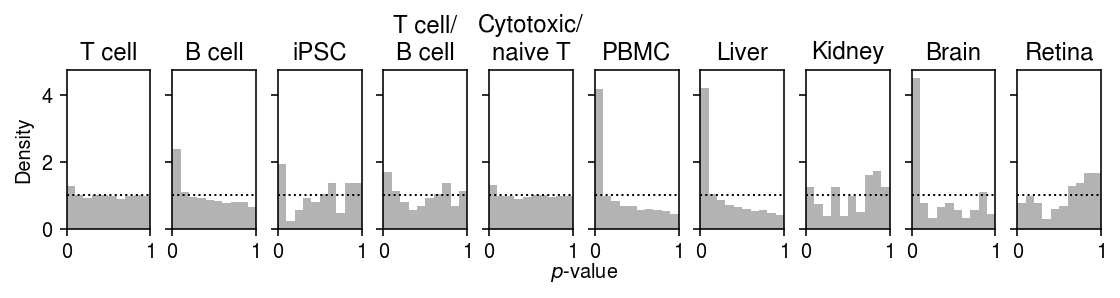
non_control = list(data.keys())[6:]
labels = ['T cell', 'B cell', 'iPSC', 'T cell/\nB cell', 'Cytotoxic/\nnaive T',
          'PBMC', 'Liver', 'Kidney', 'Brain', 'Retina']
Plot the histogram of goodness of fit test \(p\)-values for the fitted Gamma distribution.
plt.clf()
fig, ax = plt.subplots(1, 10, sharex=True, sharey=True)
fig.set_size_inches(8, 2.5)
for a, t, (k, g) in zip(ax.ravel(),
                        labels,
                        gof_res.groupby('dataset')):
  a.hist(g.loc[g['method'] == 'gamma', 'p'], bins=np.linspace(0, 1, 11), color='0.7', density=True)
  a.axhline(y=1, c='k', ls=':', lw=1)
  a.set_xlim([0, 1])
  a.set_title(t)
ax[0].set_ylabel('Density')
a = fig.add_subplot(111, xticks=[], yticks=[], frameon=False)
a.set_xlabel('$p$-value', labelpad=16)
fig.tight_layout(w_pad=0)
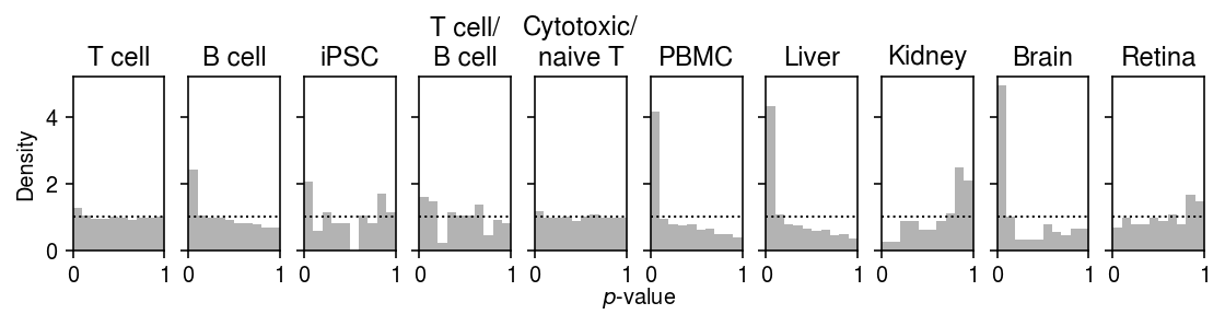
Plot the histogram of goodness of fit test \(p\)-values for the fitted point-Gamma distribution.
plt.clf()
fig, ax = plt.subplots(1, 10, sharex=True, sharey=True)
fig.set_size_inches(8, 2.5)
for a, t, (k, g) in zip(ax.ravel(),
                        labels,
                        gof_res.groupby('dataset')):
  a.hist(g.loc[g['method'] == 'zig', 'p'], bins=np.linspace(0, 1, 11), color='0.7', density=True)
  a.axhline(y=1, c='k', ls=':', lw=1)
  a.set_xlim([0, 1])
  a.set_title(t)
ax[0].set_ylabel('Density')
a = fig.add_subplot(111, xticks=[], yticks=[], frameon=False)
a.set_xlabel('$p$-value', labelpad=16)
fig.tight_layout(w_pad=0)
Report the number of genes which depart from the fitted distribution (after Bonferroni correction at level 0.05). Note the unimodal assumption was tested only for genes which significantly depart from Gamma.
(gof_res.loc[gof_res['dataset'].isin(non_control)]
 .groupby(['dataset', 'method'])
 .apply(lambda x: (x['p'] <= 0.05 / x.shape[0]).sum())
 .reset_index()
 .pivot(index='dataset', columns='method')
 [0]
 [['gamma', 'zig', 'unimodal', 'npmle']])
method               gamma   zig  unimodal  npmle
dataset
b_cells                 53    45        10     10
brain                  399   400        63     74
cytotoxic_t-b_cells   1077  1070        19     31
cytotoxic_t-naive_t    945   951        17     24
ipsc                  2246  2245         6     11
kidney                 126   122        57     66
liver-caudate-lobe      45    45         3      7
pbmcs_68k              422   409        22     48
retina                 226   202       133    125
Report the fraction of genes which do not depart from the null that the data for the gene follows the fitted distribution (after Bonferroni correction at level 0.05).
frac = (gof_res.loc[gof_res['dataset'].isin(non_control)]
        .groupby(['dataset', 'method'])
        .apply(lambda x: (x['p'] >= 0.05 / x.shape[0]).mean())
        .reset_index()
        .pivot(index='dataset', columns='method'))[0]
frac[['gamma', 'zig', 'unimodal', 'npmle']]
method                  gamma       zig  unimodal     npmle
dataset
b_cells              0.991741  0.992987  0.811321  0.811321
brain                0.966025  0.965940  0.842105  0.814536
cytotoxic_t-b_cells  0.837972  0.839025  0.982358  0.971216
cytotoxic_t-naive_t  0.848703  0.847743  0.982011  0.974603
ipsc                 0.774430  0.774530  0.997335  0.995113
kidney               0.991869  0.992127  0.547619  0.476190
liver-caudate-lobe   0.997222  0.997222  0.933333  0.844444
pbmcs_68k            0.935097  0.937096  0.947867  0.886256
retina               0.977506  0.979894  0.411504  0.446903
Remark We previously fit point-Gamma distributions to the iPSC data (Sarkar et al. 2019), and reported:
We tested the goodness of fit for each individual and each gene, and rejected the null that the model fit the data for only 60 of 537,658 individual-gene combinations (0.01%) after Bonferroni correction (\(p < 9 \times 10^{−8}\))
The key difference between the approach taken here and the previous result is that here we do not account for the fact that the cells are derived from multiple donors. The differing genetic backgrounds of the donor individuals means both the mean and variance of gene expression vary, such that the marginal distribution is not well-described by a single Gamma distribution.
Report the fraction of genes which depart from a Gamma assumption, but not a point-Gamma assumption on expression variation.
query = (gof_res[gof_res['dataset'].isin(non_control)]
         .pivot_table(index=['dataset', 'gene'], columns=['method'], values=['p', 'stat']))
(query
 .groupby(level=0)
 .apply(lambda x: np.logical_and(x['p']['gamma'] < .05 / x.shape[0],
                                 x['p']['zig'] >= .05 / x.shape[0]).sum()
        / (x['p']['gamma'] < .05 / x.shape[0]).sum()))
dataset
b_cells                0.150943
brain                  0.082707
cytotoxic_t-b_cells    0.053853
cytotoxic_t-naive_t    0.067725
ipsc                   0.000000
kidney                 0.174603
liver-caudate-lobe     0.044444
pbmcs_68k              0.099526
retina                 0.230088
dtype: float64
Report the fraction of genes which depart from a unimodal assumption, but not a fully non-parametric assumption on expression variation.
query = (gof_res[(gof_res['dataset'].isin(non_control)) & (gof_res['method'].isin(['unimodal', 'npmle']))]
         .pivot_table(index=['dataset', 'gene'], columns=['method'], values=['p', 'stat']))
(query
 .groupby(level=0)
 .apply(lambda x: np.logical_and(x['p']['unimodal'] < .05 / x.shape[0],
                                 x['p']['npmle'] >= .05 / x.shape[0]).sum()))
dataset
b_cells                 2
brain                   7
cytotoxic_t-b_cells    13
cytotoxic_t-naive_t     4
ipsc                    2
kidney                  6
liver-caudate-lobe      3
pbmcs_68k               1
retina                 20
dtype: int64
Report the number of genes where the log likelihood difference between the non-parametric expression model and unimodal model exceeds \(t \in (1, 10, 100, 1000)\), for genes which departed from a unimodal assumption on expression variation.
llr = pd.concat({k: pd.read_csv(f'/project2/mstephens/aksarkar/projects/singlecell-modes/data/gof/{k}-llr.txt.gz', sep='\t', index_col=0) for k in non_control}).reset_index()
llr.groupby('level_0').apply(lambda x: pd.Series({t: (x['llr'] > t).sum() for t in (1, 10, 100, 1000)}))
1     10    100   1000
level_0
b_cells                 6     1     0     0
brain                  52     3     1     1
cytotoxic_t-b_cells    49    16     6     1
cytotoxic_t-naive_t    30     1     0     0
ipsc                  542    12     2     0
kidney                 51     2     0     0
liver-caudate-lobe     28    12     1     0
pbmcs_68k              66    12     1     0
retina                 74    20     9     0
Report the intersection of the two sets of putative multi-modal genes.
sig = (gof_res
       .pivot_table(index=['dataset', 'gene'], columns=['method'], values=['p'])
       ['p']
       .groupby(level=0)
       .apply(lambda x: x.loc[(x['unimodal'] < 0.05 / x.shape[0]) & (x['npmle'] >= 0.05 / x.shape[0])])
       .reset_index(level=0, drop=True)
       .reset_index()
)
query = (sig
         .merge(llr.loc[llr['llr'] > 10], left_on=['dataset', 'gene'], right_on=['level_0', 'gene'])
         .reset_index(drop=True)
         .merge(gene_info, on='gene'))
query.shape
(20, 15)
Browser
Read gene metadata.
gene_info = pd.read_csv('/project2/mstephens/aksarkar/projects/singlecell-qtl/data/scqtl-genes.txt.gz', sep='\t', index_col=0)
Populate the database with the genes departing from a unimodal expression model.
sig = (gof_res
       .pivot_table(index=['dataset', 'gene'], columns=['method'], values=['p'])
       ['p']
       .groupby(level=0)
       .apply(lambda x: x.loc[(x['unimodal'] < 0.05 / x.shape[0]) & (x['npmle'] >= 0.05 / x.shape[0])])
       .reset_index(level=0, drop=True)
       .reset_index()
)
dat = (sig
         .merge(llr.loc[llr['llr'] > 10], left_on=['dataset', 'gene'], right_on=['level_0', 'gene'], how='outer')
         .reset_index(drop=True)
         .merge(gene_info, on='gene'))
dat['dataset'].fillna(dat['level_0'], inplace=True)
dat = dat[['dataset', 'gene', 'name', 'unimodal', 'npmle', 'llr']]
keys = []
counts = []
for k, g in dat.groupby(['dataset']):
  x = data[k]()
  query = g['gene'].unique()
  if not isinstance(x, anndata.AnnData):
    counts.append(x[query])
  else:
    key = [t for t in ('gene', 'ID', 'featurekey', 0) if t in x.var.columns][0]
    counts.append(pd.DataFrame(x[:,x.var[key].isin(query)].X.A, index=x.obs.index, columns=query))
  keys.append(k)

def _melt(y):
  y.index.name = 'sample'
  return (y
          .reset_index()
          .melt(id_vars='sample', var_name='gene', value_name='count'))

count_data = (pd.concat([_melt(y) for y in counts], keys=keys)
              .reset_index(level=0)
              .rename({'level_0': 'dataset'}, axis=1))
with sqlite3.connect('/project2/mstephens/aksarkar/projects/singlecell-modes/browser/browser.db') as conn:
  dat.to_sql('genes', conn, if_exists='replace', index=False)
  conn.execute('create index genes_idx on genes(dataset, gene);')
  count_data.to_sql('counts', conn, if_exists='replace', index=False)
  conn.execute('create index counts_idx on counts(dataset, gene);')
Real data examples
Read the results.
gene_info = pd.read_csv('/project2/mstephens/aksarkar/projects/singlecell-qtl/data/scqtl-genes.txt.gz', sep='\t', index_col=0)
gof_res = pd.read_csv('/project2/mstephens/aksarkar/projects/singlecell-modes/data/gof/gof.txt.gz', sep='\t', index_col=0)
sig = (gof_res
       .loc[gof_res['method'] == 'unimodal']
       .groupby('dataset')
       .apply(lambda x: x.loc[x['p'] < 0.05 / x.shape[0]].sort_values('p').head(n=100))
       .reset_index(drop=True)
       .merge(gene_info, on='gene', how='left')
       [['dataset', 'gene', 'name', 'method', 'stat', 'p']])
Get examples of genes which significantly depart from the estimated unimodal distribution, but are clearly unimodal upon inspection.
dat = anndata.read_h5ad('/scratch/midway2/aksarkar/modes/unimodal-data/b_cells.h5ad')
Write out the data to RDS.
rpy2.robjects.r['saveRDS'](
  pd.DataFrame(dat.X, columns=dat.var.index, index=dat.obs.index)
  .reset_index()
  .rename({'index': 'sample'}, axis=1)
  .melt(id_vars='sample', var_name='gene', value_name='count')
  .merge(dat.obs, left_on='sample', right_index=True)
  .sort_values(['gene', 'sample'])
  .reset_index(drop=True),
  'b-cell-data.Rds')
rpy2.rinterface.NULL
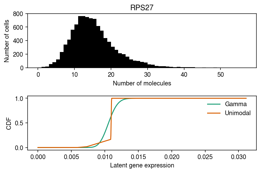
RPS27 departs from Gamma, point-Gamma, and unimodal.
query = list(dat.var.index).index(sig.loc[sig['dataset'] == 'b_cells', 'gene'].head(n=1)[0])
cm = plt.get_cmap('Dark2')
plt.clf()
fig, ax = plt.subplots(2, 1)
fig.set_size_inches(6, 4)

ax[0].hist(dat.X[:,query], bins=np.arange(dat.X[:,query].max() + 1), color='k')
ax[0].set_xlabel('Number of molecules')
ax[0].set_ylabel('Number of cells')
ax[0].set_title(gene_info.loc[dat.var.index[query], 'name'])

for i, m in enumerate(('gamma', 'unimodal')):
  ax[1].plot(*getattr(scmodes.deconvolve, f'fit_{m}')(dat.X[:,query], dat.obs['size']), c=cm(i), label=m.capitalize())
ax[1].legend(frameon=False)
ax[1].set_xlabel('Latent gene expression')
ax[1].set_ylabel('CDF')
fig.tight_layout()
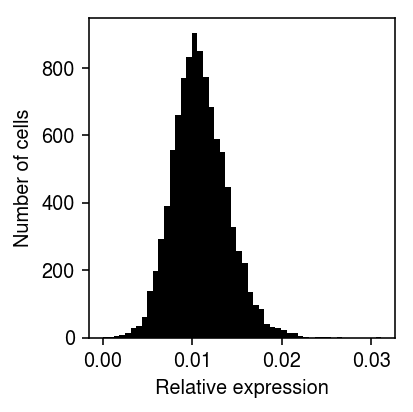
Look at the distribution of the MLE \(\hat\lambda_i = x_i / s_i\) (intuitively, the quantity which we will be shrinking).
plt.clf()
plt.gcf().set_size_inches(3, 3)
plt.hist(dat.X[:,query] / dat.obs['size'], bins=50, color='k')
plt.xlabel('Relative expression')
plt.ylabel('Number of cells')
plt.tight_layout()
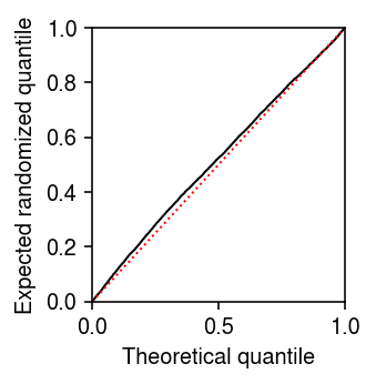
Repeat the test for goodness of fit for the fitted unimodal distribution.
unimodal_res = scmodes.ebpm.ebpm_unimodal(dat.X[:,query], dat.obs['size'].values)
F = scmodes.benchmark.gof._ash_cdf(dat.X[:,query] - 1, fit=unimodal_res, s=dat.obs['size'])
f = scmodes.benchmark.gof._ash_pmf(dat.X[:,query], fit=unimodal_res, s=dat.obs['size'])
np.random.seed(0)
rpp = F + np.random.uniform(size=f.shape) * f
st.kstest(rpp, 'uniform')
KstestResult(statistic=0.03257412894279588, pvalue=1.0146593403454815e-09)
Look at the expected randomized quantiles.
plt.clf()
plt.gcf().set_size_inches(2.5, 2.5)
plt.plot(np.linspace(0, 1, rpp.shape[0] + 2)[1:-1], np.sort(F + .5 * f), lw=1, c='k')
lim = [0, 1]
plt.plot(lim, lim, lw=1, ls=':', c='r')
plt.xlim(lim)
plt.ylim(lim)
plt.xlabel('Theoretical quantile')
plt.ylabel('Expected randomized quantile')
plt.tight_layout()
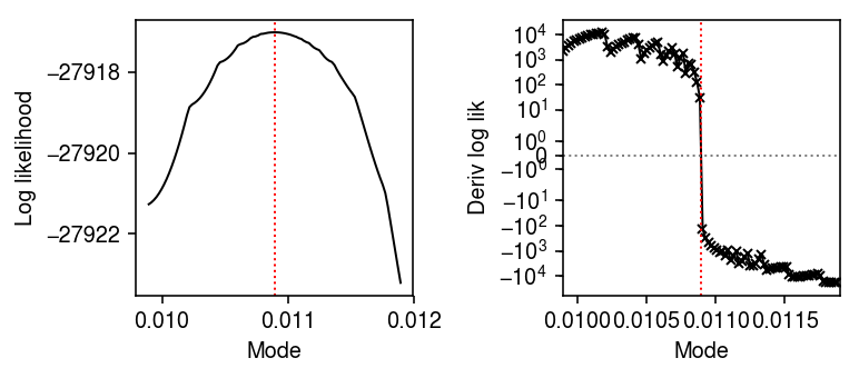
Look at the mode search subproblem.
lam = dat.X[:,query] / dat.obs['size']
res0 = scmodes.ebpm.ebpm_unimodal(dat.X[:,query], dat.obs['size'].values)
mode = np.array(res0.rx2('fitted_g').rx2('a'))[0]
grid = np.linspace(mode - 1e-3, mode + 1e-3, 100)
res = pd.DataFrame.from_dict(
  {m: np.array(scmodes.ebpm.ebpm_unimodal(dat.X[:,query], dat.obs['size'], mode=m).rx2('loglik'))
   for m in grid},
  orient='index')
plt.clf()
fig, ax = plt.subplots(1, 2)
fig.set_size_inches(5.5, 2.5)
ax[0].plot(grid, res[0], lw=1, c='k')
ax[0].set_ylabel('Log likelihood')

ax[1].set_xlim(mode - 1e-3, mode + 1e-3)
ax[1].set_yscale('symlog')
ax[1].plot(grid[:-1], np.diff(res[0]) / np.diff(grid), marker='x', ms=4, lw=1, c='k')
ax[1].axhline(y=0, lw=1, ls=':', c='0.5')
ax[1].set_ylabel('Deriv log lik')
for a in ax:
  a.axvline(x=mode, lw=1, ls=':', c='r')
  a.set_xlabel('Mode')
fig.tight_layout()
Fit models with finer grids.
res = dict()
for step in np.log(np.linspace(1, 2, 11)[1:]):
  res[step] = scmodes.ebpm.ebpm_unimodal(
    dat.X[:,0],
    dat.obs['size'],
    mixsd=np.exp(np.arange(np.log(1e-8), np.log(lam.max()), step=step)))
Report the log likelihood of the fitted models against the (log) stepsize of the grid.
pd.Series({k: np.array(res[k].rx2('loglik'))[0] for k in res})
0.095310   -27916.693078
0.182322   -27916.691828
0.262364   -27916.847090
0.336472   -27917.009390
0.405465   -27916.711257
0.470004   -27917.364408
0.530628   -27917.541988
0.587787   -27917.067727
0.641854   -27917.669822
0.693147   -27918.161042
dtype: float64
Test the fitted models for goodness of fit, and report the KS test statistic and \(p\)-value.
np.random.seed(1)
pd.Series({
  k: scmodes.benchmark.gof._gof(
    dat.X[:,0],
    cdf=scmodes.benchmark.gof._ash_cdf,
    pmf=scmodes.benchmark.gof._ash_pmf,
    s=dat.obs['size'],
    fit=res[k])
  for k in res})
0.095310     (0.03343639916233043, 3.219041220233783e-10)
0.182322     (0.03349651214950944, 2.968120165176161e-10)
0.262364     (0.03281679008032623, 7.367539493197478e-10)
0.336472      (0.03312928499093126, 4.86187521991659e-10)
0.405465     (0.03260696496636967, 9.717889023225659e-10)
0.470004    (0.03257735474891127, 1.0103672529713676e-09)
0.530628    (0.033042770023911816, 5.456976614561023e-10)
0.587787     (0.03396250448855004, 1.574404486410344e-10)
0.641854    (0.03380000822864859, 1.9659431226291915e-10)
0.693147    (0.034306982158272215, 9.797409099464328e-11)
dtype: object
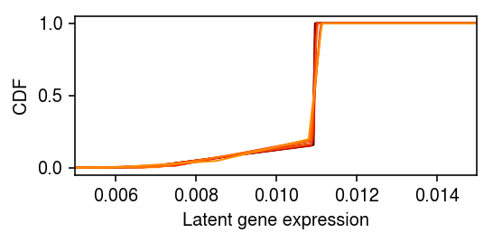
Look at the fitted distributions.
plt.clf()
plt.gcf().set_size_inches(4, 2)
grid = np.linspace(lam.min(), lam.max(), 1000)
for k in res:
  F = ashr.cdf_ash(res[k], grid)
  plt.plot(grid, np.array(F.rx2('y')).ravel(), c=colorcet.cm['fire'](k), lw=1)
plt.xlim(.005, .015)
plt.xlabel('Latent gene expression')
plt.ylabel('CDF')
plt.tight_layout()
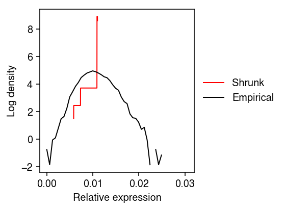
Overlay the estimated density with the empirical density of the naive MLE.
grid = np.linspace(lam.min(), lam.max(), 5000)
F = ashr.cdf_ash(res0, grid)
f = np.diff(np.array(F.rx2('y')).ravel()) / np.diff(grid)

plt.clf()
plt.gcf().set_size_inches(4, 3)
plt.plot(grid[:-1], np.log(f), c='r', lw=1, label='Shrunk')
h = np.histogram(dat.X[:,query] / dat.obs['size'], density=True, bins=50)
plt.plot(h[1][:-1], np.log(h[0]), c='k', lw=1, label='Empirical')
plt.legend(frameon=False, loc='center left', bbox_to_anchor=(1, .5))
plt.xlabel('Relative expression')
plt.ylabel('Log density')
plt.tight_layout()
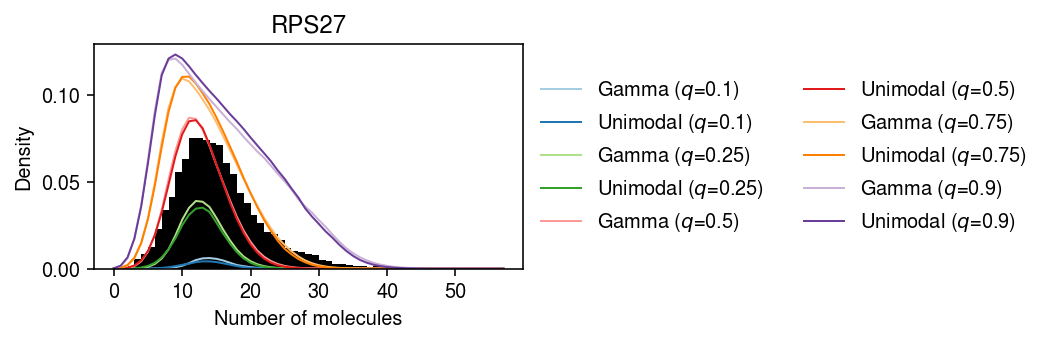
Plot the (average) marginal density over the observed data.
\begin{align} \Pr(x = k) &= E_{x_{i+} \sim \hat{p}(x_{i+})}[\Pr(x = k \mid x_{i+})]\\ &= \frac{1}{n} \sum_i \int_0^{\infty} \operatorname{Poisson}(k; x_{i+} \lambda\)\, dg(\lambda) \end{align}pmf = dict() gamma_res = scmodes.ebpm.ebpm_gamma(x, s) x = dat.X[:,query] s = dat.obs['size'] y = np.arange(x.max() + 1) g = np.array(res.rx2('fitted_g')) a = np.fmin(g[1], g[2]) b = np.fmax(g[1], g[2]) for q in (.1, .25, .5, .75, .9): pmf[f'Gamma ($q$={q})'] = np.array([np.percentile(scmodes.benchmark.gof._zig_pmf(k, size=s, log_mu=gamma_res[0], log_phi=-gamma_res[1]), 100 * q) for k in y]) comp_dens_conv = np.array([np.percentile(((st.gamma(a=k + 1, scale=1 / s.values.reshape(-1, 1)).cdf(b.reshape(1, -1)) - st.gamma(a=k + 1, scale=1 / s.values.reshape(-1, 1)).cdf(a.reshape(1, -1))) / np.outer(s, b - a)), 100 * q, axis=0) for k in y]) comp_dens_conv[:,0] = np.percentile(st.poisson(mu=s.values.reshape(-1, 1) * b[0]).pmf(y), 100 * q, axis=0) pmf[f'Unimodal ($q$={q})'] = comp_dens_conv @ g[0]
cm = plt.get_cmap('Paired')
plt.clf()
plt.gcf().set_size_inches(7.5, 2.5)
plt.hist(dat.X[:,query], bins=np.arange(dat.X[:,query].max() + 1), color='k', density=True)
for i, k in enumerate(pmf):
  plt.plot(y, pmf[k], c=cm(i), lw=1, label=k)
plt.legend(frameon=False, loc='center left', bbox_to_anchor=(1, .5), ncol=2)
plt.xlabel('Number of molecules')
plt.ylabel('Density')
plt.title(gene_info.loc[dat.var.index[query], 'name'])
plt.tight_layout()
One possibility is that the departure from the fitted distribution is caused by the assumption that \(g\) does not depend on \(x_{i+}\). First, fit a fully non-parametric model and test for goodness of fit.
npmle_res = scmodes.ebpm.ebpm_npmle(dat.X[:,query], dat.obs['size'].values)
F = scmodes.benchmark.gof._ash_cdf(dat.X[:,query] - 1, fit=npmle_res, s=dat.obs['size'])
f = scmodes.benchmark.gof._ash_pmf(dat.X[:,query], fit=npmle_res, s=dat.obs['size'])
np.random.seed(0)
rpp = F + np.random.uniform(size=f.shape) * f
st.kstest(rpp, 'uniform')
KstestResult(statistic=0.03233198676384014, pvalue=1.3931326313216651e-09)
Compare the log likelihoods of the fit.
(np.array(npmle_res.rx2('loglik')) - np.array(unimodal_res.rx2('loglik')))[0]
1.0301746905533946
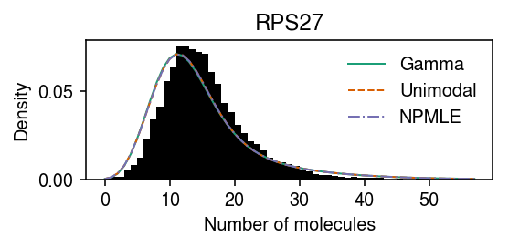
Plot the average density.
pmf = dict()
x = dat.X[:,query]
s = dat.obs['size']
y = np.arange(x.max() + 1)

gamma_res = scmodes.ebpm.ebpm_gamma(x, s)
pmf[f'Gamma'] = np.array([scmodes.benchmark.gof._zig_pmf(k, size=s, log_mu=gamma_res[0], log_phi=-gamma_res[1]).mean(axis=0) for k in y])

g = np.array(unimodal_res.rx2('fitted_g'))
a = np.fmin(g[1], g[2])
b = np.fmax(g[1], g[2])
comp_dens_conv = np.array([((st.gamma(a=k + 1, scale=1 / s.values.reshape(-1, 1)).cdf(b.reshape(1, -1)) - st.gamma(a=k + 1, scale=1 / s.values.reshape(-1, 1)).cdf(a.reshape(1, -1))) / np.outer(s, b - a)).mean(axis=0) for k in y])
comp_dens_conv[:,0] = st.poisson(mu=s.values.reshape(-1, 1) * b[0]).pmf(y).mean(axis=0)
pmf[f'Unimodal'] = comp_dens_conv @ g[0]

g = np.array(npmle_res.rx2('fitted_g'))
a = np.fmin(g[1], g[2])
b = np.fmax(g[1], g[2])
comp_dens_conv = np.array([((st.gamma(a=k + 1, scale=1 / s.values.reshape(-1, 1)).cdf(b.reshape(1, -1)) - st.gamma(a=k + 1, scale=1 / s.values.reshape(-1, 1)).cdf(a.reshape(1, -1))) / np.outer(s, b - a)).mean(axis=0) for k in y])
comp_dens_conv[:,0] = st.poisson(mu=s.values.reshape(-1, 1) * b[0]).pmf(y).mean(axis=0)
pmf[f'NPMLE'] = comp_dens_conv @ g[0]
cm = plt.get_cmap('Dark2')
plt.clf()
plt.gcf().set_size_inches(4, 2)
plt.hist(dat.X[:,query], bins=np.arange(dat.X[:,query].max() + 1), color='k', density=True)
for i, (k, ls) in enumerate(zip(pmf, ['-', '--', '-.'])):
  plt.plot(y, pmf[k], c=cm(i), lw=1, ls=ls, label=k)
plt.legend(frameon=False)
plt.xlabel('Number of molecules')
plt.ylabel('Density')
plt.title(gene_info.loc[dat.var.index[query], 'name'])
plt.tight_layout()
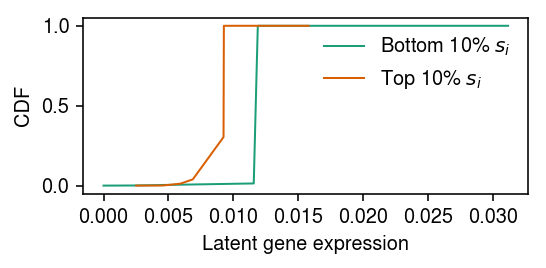
Fit two expression models, one to the 10% of samples with smallest \(x_{i+}\), and one to the 10% of samples with largest \(x_{i+}\), then compare the fitted models.
cm = plt.get_cmap('Dark2')
order = np.argsort(s.values)
low_pass = order[:1000]
high_pass = order[-1000:]
plt.clf()
plt.gcf().set_size_inches(4, 2)
plt.plot(*getattr(scmodes.deconvolve, f'fit_unimodal')(x[low_pass], s.values[low_pass]), c=cm(0), lw=1, label='Bottom 10% $s_i$')
plt.plot(*getattr(scmodes.deconvolve, f'fit_unimodal')(x[high_pass], s.values[high_pass]), c=cm(1), lw=1, label='Top 10% $s_i$')
plt.legend(frameon=False)
plt.xlabel('Latent gene expression')
plt.ylabel('CDF')
plt.tight_layout()
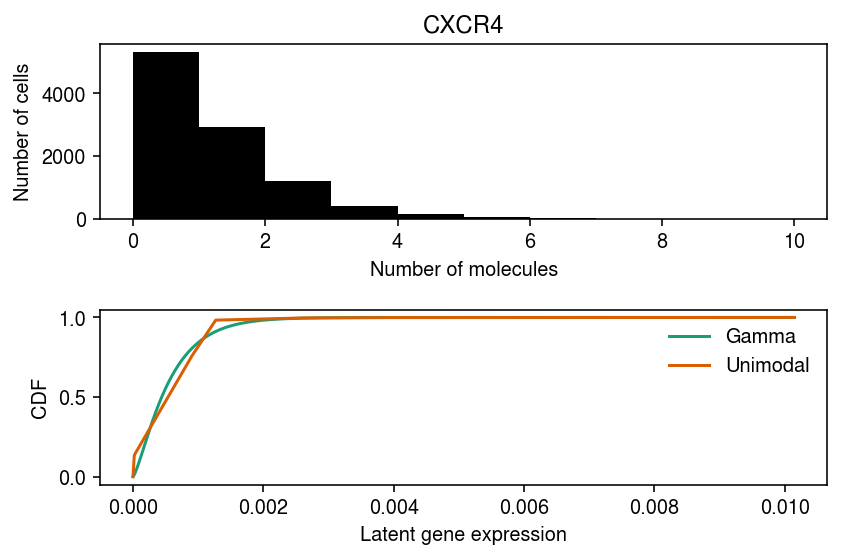
CXCR4 departs from Gamma, but not from point-Gamma.
cm = plt.get_cmap('Dark2')
plt.clf()
fig, ax = plt.subplots(2, 1)
fig.set_size_inches(6, 4)

ax[0].hist(dat.X[:,1], bins=np.arange(dat.X[:,1].max() + 1), color='k')
ax[0].set_xlabel('Number of molecules')
ax[0].set_ylabel('Number of cells')
ax[0].set_title(gene_info.loc[dat.var.index[1], 'name'])

for i, m in enumerate(('gamma', 'unimodal')):
  ax[1].plot(*getattr(scmodes.deconvolve, f'fit_{m}')(dat.X[:,1], dat.obs['size']), c=cm(i), label=m.capitalize())
ax[1].legend(frameon=False)
ax[1].set_xlabel('Latent gene expression')
ax[1].set_ylabel('CDF')
fig.tight_layout()
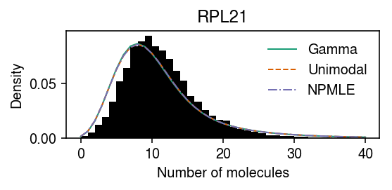
RPL21 departed from NPMLE, but not unimodal.
query = (gof_res
         .groupby(["dataset", "method"])
         .apply(lambda x: x.loc[x['p'] < 0.05 / x.shape[0]])
         .reset_index(drop=True)
         .pivot_table(index=['dataset', 'gene'], columns='method', values='p'))
query = (query
         .loc[np.isfinite(query['npmle']) & ~np.isfinite(query['unimodal'])]
         .reset_index()
         .head(n=1)
         ['gene'][0])
query = list(dat.var.index).index(query)
29
pmf = dict()
x = dat.X[:,query]
s = dat.obs['size']
y = np.arange(x.max() + 1)

gamma_res = scmodes.ebpm.ebpm_gamma(x, s)
pmf[f'Gamma'] = np.array([scmodes.benchmark.gof._zig_pmf(k, size=s, log_mu=gamma_res[0], log_phi=-gamma_res[1]).mean(axis=0) for k in y])

unimodal_res = scmodes.ebpm.ebpm_unimodal(dat.X[:,query], dat.obs['size'].values)
g = np.array(unimodal_res.rx2('fitted_g'))
a = np.fmin(g[1], g[2])
b = np.fmax(g[1], g[2])
comp_dens_conv = np.array([((st.gamma(a=k + 1, scale=1 / s.values.reshape(-1, 1)).cdf(b.reshape(1, -1)) - st.gamma(a=k + 1, scale=1 / s.values.reshape(-1, 1)).cdf(a.reshape(1, -1))) / np.outer(s, b - a)).mean(axis=0) for k in y])
comp_dens_conv[:,0] = st.poisson(mu=s.values.reshape(-1, 1) * b[0]).pmf(y).mean(axis=0)
pmf[f'Unimodal'] = comp_dens_conv @ g[0]

npmle_res = scmodes.ebpm.ebpm_npmle(dat.X[:,query], dat.obs['size'].values)
g = np.array(npmle_res.rx2('fitted_g'))
a = np.fmin(g[1], g[2])
b = np.fmax(g[1], g[2])
comp_dens_conv = np.array([((st.gamma(a=k + 1, scale=1 / s.values.reshape(-1, 1)).cdf(b.reshape(1, -1)) - st.gamma(a=k + 1, scale=1 / s.values.reshape(-1, 1)).cdf(a.reshape(1, -1))) / np.outer(s, b - a)).mean(axis=0) for k in y])
comp_dens_conv[:,0] = st.poisson(mu=s.values.reshape(-1, 1) * b[0]).pmf(y).mean(axis=0)
pmf[f'NPMLE'] = comp_dens_conv @ g[0]
cm = plt.get_cmap('Dark2')
plt.clf()
plt.gcf().set_size_inches(4, 2)
plt.hist(dat.X[:,query], bins=np.arange(dat.X[:,query].max() + 1), color='k', density=True)
for i, (k, ls) in enumerate(zip(pmf, ['-', '--', '-.'])):
  plt.plot(y, pmf[k], c=cm(i), lw=1, ls=ls, label=k)
plt.legend(frameon=False)
plt.xlabel('Number of molecules')
plt.ylabel('Density')
plt.title(gene_info.loc[dat.var.index[query], 'name'])
plt.tight_layout()