Comparison of fitted values
Table of Contents
Introduction
We previously found that NMF, GLM-PCA, and PVAE all had similar average performance on a binomial thinning benchmark. Here, we investigate the per-observation performance of these methods.
Setup
import anndata
import numpy as np
import pandas as pd
import scanpy as sc
import scipy.stats as st
import scmodes
import torch
%matplotlib inline
%config InlineBackend.figure_formats = set(['retina'])
import matplotlib.pyplot as plt
plt.rcParams['figure.facecolor'] = 'w'
plt.rcParams['font.family'] = 'Nimbus Sans'
Results
Datasets
Follow the data processing for the Poisson thinning analysis.
B cells
Split the data into training and validation sets using binomial thinning, then fit NMF, GLMPCA, and PVAE.
# Important: this implicitly sets the random seed
x = data['b_cells']()
train, test = scmodes.benchmark.train_test_split(x)
np.save('/scratch/midway2/aksarkar/modes/fitted-values/b_cells-train', train)
np.save('/scratch/midway2/aksarkar/modes/fitted-values/b_cells-test', test)
sbatch --partition=broadwl -n1 --mem=8G --time=24:00:00
#!/bin/bash
source activate scmodes
python <<EOF
<<imports>>
train = np.load('/scratch/midway2/aksarkar/modes/fitted-values/b_cells-train.npy')
l, f, _ = scmodes.lra.nmf(train, rank=8, tol=1e-2, max_iters=100000, verbose=True)
lam0 = l @ f.T
np.save('/scratch/midway2/aksarkar/modes/fitted-values/b_cells-nmf-lam', lam0)

l, f, _ = scmodes.lra.glmpca(train, rank=8, tol=1e-2, max_iters=100000, verbose=True)
lam1 = np.exp(l @ f.T)
np.save('/scratch/midway2/aksarkar/modes/fitted-values/b_cells-glmpca-lam', lam1)
EOF
sbatch --partition=gpu2 --gres=gpu:1 --mem=8G
#!/bin/bash
source activate scmodes
python <<EOF
<<imports>>
train = np.load('/scratch/midway2/aksarkar/modes/fitted-values/b_cells-train.npy')
torch.manual_seed(1)
xt = torch.tensor(train, dtype=torch.float)
m = scmodes.lra.PVAE(input_dim=train.shape[1], latent_dim=8).fit(xt, test_size=0.1, lr=1e-3, max_epochs=200, trace=True)
lam2 = m.denoise(xt, n_samples=100)
np.save('/scratch/midway2/aksarkar/modes/fitted-values/b_cells-pvae-lam', lam2)
np.save('/scratch/midway2/aksarkar/modes/fitted-values/b_cells-pvae-trace', np.array(m.trace))

m = scmodes.lra.NBVAE(input_dim=train.shape[1], latent_dim=8, disp_by_gene=True).fit(xt, test_size=0.1, lr=1e-3, max_epochs=400, trace=True)
lam3 = m.denoise(xt, n_samples=100)
np.save('/scratch/midway2/aksarkar/modes/fitted-values/b_cells-nbvae-log_inv_disp',
        m.log_inv_disp.detach().cpu().numpy())
np.save('/scratch/midway2/aksarkar/modes/fitted-values/b_cells-nbvae-lam', lam3)
np.save('/scratch/midway2/aksarkar/modes/fitted-values/b_cells-nbvae-trace', np.array(m.trace))
EOF
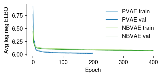
Examine the VAE optimization traces.
cm = plt.get_cmap('Paired')
plt.clf()
plt.gcf().set_size_inches(4, 2)
trace = np.load('/scratch/midway2/aksarkar/modes/fitted-values/b_cells-pvae-trace.npy')
trace2 = np.load('/scratch/midway2/aksarkar/modes/fitted-values/b_cells-nbvae-trace.npy')
for i, (t, s, k) in enumerate(zip(trace.T, [900, 100], ['PVAE train', 'PVAE val'])):
  plt.plot(np.log(t / s), lw=1, c=cm(i), label=k)
for i, (t, s, k) in enumerate(zip(trace2.T, [900, 100], ['NBVAE train', 'NBVAE val'])):
  plt.plot(np.log(t / s), lw=1, c=cm(i + 2), label=k)
plt.legend(frameon=False)
plt.xlabel('Epoch')
plt.ylabel('Avg log neg ELBO')
plt.tight_layout()
Read the results.
train = np.load('/scratch/midway2/aksarkar/modes/fitted-values/b_cells-train.npy')
test = np.load('/scratch/midway2/aksarkar/modes/fitted-values/b_cells-test.npy')
lam0 = np.load('/scratch/midway2/aksarkar/modes/fitted-values/b_cells-nmf-lam.npy')
lam1 = np.load('/scratch/midway2/aksarkar/modes/fitted-values/b_cells-glmpca-lam.npy')
lam2 = np.load('/scratch/midway2/aksarkar/modes/fitted-values/b_cells-pvae-lam.npy')
lam3 = np.load('/scratch/midway2/aksarkar/modes/fitted-values/b_cells-nbvae-lam.npy')
nbvae_log_inv_disp = np.load('/scratch/midway2/aksarkar/modes/fitted-values/b_cells-nbvae-log_inv_disp.npy')
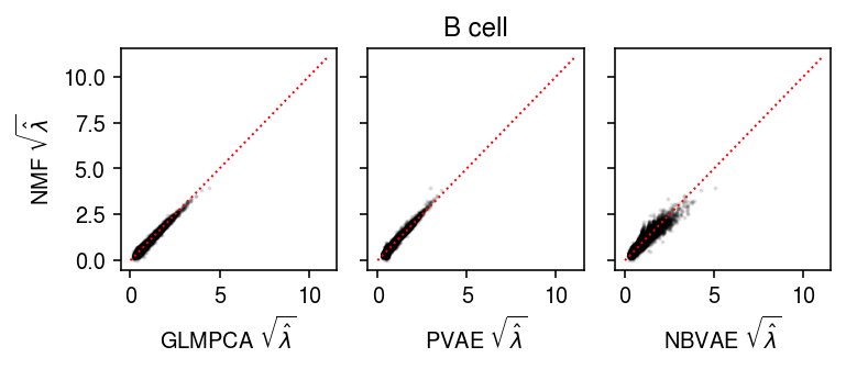
Compare the fitted values of each method against other.
plt.clf()
fig, ax = plt.subplots(1, 3, sharey=True)
fig.set_size_inches(5.5, 2.5)

ax[0].scatter(np.sqrt(lam1.ravel()[::50]), np.sqrt(lam0.ravel()[::50]), s=1, c='k', alpha=0.1)
ax[0].plot([0, 11], [0, 11], lw=1, ls=':', c='r')
ax[0].set_xlabel(r'GLMPCA $\sqrt{\hat\lambda}$')
ax[0].set_ylabel(r'NMF $\sqrt{\hat\lambda}$')

ax[1].scatter(np.sqrt(lam2.ravel()[::50]), np.sqrt(lam0.ravel()[::50]), s=1, c='k', alpha=0.1)
ax[1].plot([0, 11], [0, 11], lw=1, ls=':', c='r')
ax[1].set_xlabel(r'PVAE $\sqrt{\hat\lambda}$')

ax[2].scatter(np.sqrt(lam3.ravel()[::50]), np.sqrt(lam0.ravel()[::50]), s=1, c='k', alpha=0.1)
ax[2].plot([0, 11], [0, 11], lw=1, ls=':', c='r')
ax[2].set_xlabel(r'NBVAE $\sqrt{\hat\lambda}$')

a = fig.add_subplot(111, frame_on=False, xticks=[], yticks=[])
a.set_title('B cell')
fig.tight_layout()
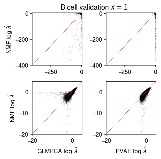
Compare the fitted values of each method against each other, only for observations which were 1 in the validation data.
plt.clf()
fig, ax = plt.subplots(2, 2)
fig.set_size_inches(4, 4)

query = np.isclose(test, 1)
lim = [-400, 5]
ax[0][0].scatter(np.log(lam1[query].ravel()), np.log(lam0[query].ravel()), s=1, c='k', alpha=0.1)
ax[0][0].plot(lim, lim, lw=1, ls=':', c='r')
ax[0][0].set_xlim(lim)
ax[0][0].set_ylim(lim)
ax[0][0].set_ylabel(r'NMF $\log\ \hat\lambda$')

ax[0][1].scatter(np.log(lam2[query].ravel()), np.log(lam0[query].ravel()), s=1, c='k', alpha=0.1)
ax[0][1].plot(lim, lim, lw=1, ls=':', c='r')
ax[0][1].set_xlim(lim)
ax[0][1].set_ylim(lim)

lim = [-20, 5]
ax[0][0].add_patch(plt.Rectangle((lim[0], lim[0]), lim[1] - lim[0], lim[1] - lim[0], fill=False, color='b'))
ax[0][1].add_patch(plt.Rectangle((lim[0], lim[0]), lim[1] - lim[0], lim[1] - lim[0], fill=False, color='b'))

ax[1][0].scatter(np.log(lam1[query].ravel()), np.log(lam0[query].ravel()), s=1, c='k', alpha=0.1)
ax[1][0].plot(lim, lim, lw=1, ls=':', c='r')
ax[1][0].set_xlim(lim)
ax[1][0].set_ylim(lim)
ax[1][0].set_xlabel(r'GLMPCA $\log\ \hat\lambda$')
ax[1][0].set_ylabel(r'NMF $\log\ \hat\lambda$')

ax[1][1].scatter(np.log(lam2[query].ravel()), np.log(lam0[query].ravel()), s=1, c='k', alpha=0.1)
ax[1][1].plot(lim, lim, lw=1, ls=':', c='r')
ax[1][1].set_xlim(lim)
ax[1][1].set_ylim(lim)
ax[1][1].set_xlabel(r'PVAE $\log\ \hat\lambda$')

a = fig.add_subplot(111, frame_on=False, xticks=[], yticks=[])
a.set_title('B cell validation $x = 1$')
fig.tight_layout()
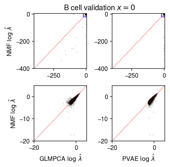
Repeat for observations which were 0 in the validation data.
plt.clf()
fig, ax = plt.subplots(2, 2)
fig.set_size_inches(4, 4)

query = np.isclose(test, 0)
lim = [-400, 5]
ax[0][0].scatter(np.log(lam1[query].ravel()[::50]), np.log(lam0[query].ravel()[::50]), s=1, c='k', alpha=0.1)
ax[0][0].plot(lim, lim, lw=1, ls=':', c='r')
ax[0][0].set_xlim(lim)
ax[0][0].set_ylim(lim)
ax[0][0].set_ylabel(r'NMF $\log\ \hat\lambda$')

ax[0][1].scatter(np.log(lam2[query].ravel()[::50]), np.log(lam0[query].ravel()[::50]), s=1, c='k', alpha=0.1)
ax[0][1].plot(lim, lim, lw=1, ls=':', c='r')
ax[0][1].set_xlim(lim)
ax[0][1].set_ylim(lim)

lim = [-20, 5]
ax[0][0].add_patch(plt.Rectangle((lim[0], lim[0]), lim[1] - lim[0], lim[1] - lim[0], fill=False, color='b'))
ax[0][1].add_patch(plt.Rectangle((lim[0], lim[0]), lim[1] - lim[0], lim[1] - lim[0], fill=False, color='b'))

ax[1][0].scatter(np.log(lam1[query].ravel()[::50]), np.log(lam0[query].ravel()[::50]), s=1, c='k', alpha=0.1)
ax[1][0].plot(lim, lim, lw=1, ls=':', c='r')
ax[1][0].set_xlim(lim)
ax[1][0].set_ylim(lim)
ax[1][0].set_xlabel(r'GLMPCA $\log\ \hat\lambda$')
ax[1][0].set_ylabel(r'NMF $\log\ \hat\lambda$')

ax[1][1].scatter(np.log(lam2[query].ravel()[::50]), np.log(lam0[query].ravel()[::50]), s=1, c='k', alpha=0.1)
ax[1][1].plot(lim, lim, lw=1, ls=':', c='r')
ax[1][1].set_xlim(lim)
ax[1][1].set_ylim(lim)
ax[1][1].set_xlabel(r'PVAE $\log\ \hat\lambda$')

a = fig.add_subplot(111, frame_on=False, xticks=[], yticks=[])
a.set_title('B cell validation $x = 0$')
fig.tight_layout()
Look at the average training log likelihoods.
llik0 = st.poisson(lam0).logpmf(train)
llik1 = st.poisson(lam1).logpmf(train)
llik2 = st.poisson(lam2).logpmf(train)
llik3 = st.poisson(lam3).logpmf(train)
pd.Series({'NMF': llik0.mean(), 'GLMPCA': llik1.mean(), 'PVAE': llik2.mean(), 'NBVAE': llik3.mean()})
NMF      -1.038913
GLMPCA   -1.036029
PVAE     -1.062526
NBVAE    -0.830541
dtype: float64
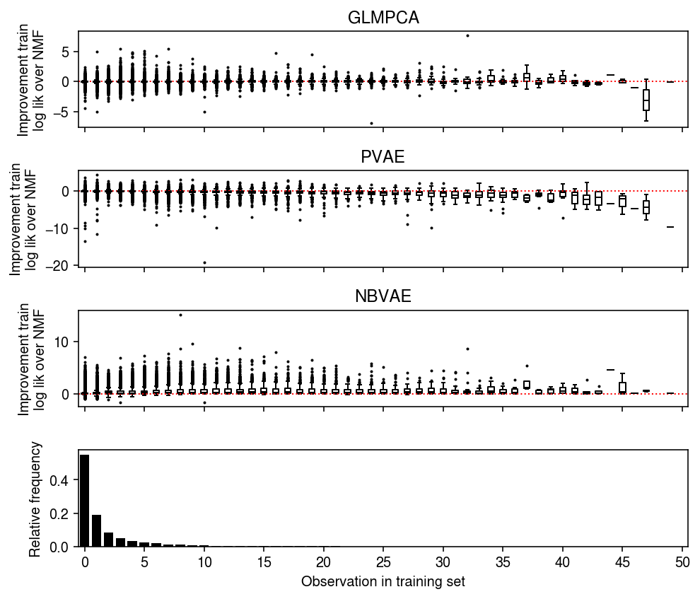
Look at the distribution of per-observation training log likelihood differences, stratified by observed value.
plt.clf()
fig, ax = plt.subplots(4, 1, sharex=True)
fig.set_size_inches(7, 6)

grid = np.arange(train.max() + 1)
for i in grid:
  ax[0].boxplot((llik1 - llik0)[train == i].ravel(), positions=[i], widths=[0.5], medianprops={'color': 'k'}, flierprops={'marker': '.', 'markersize': 2})
ax[0].axhline(y=0, ls=':', lw=1, c='r')
ax[0].set_ylabel('Improvement train\nlog lik over NMF')
ax[0].set_title('GLMPCA')

for i in grid:
  ax[1].boxplot((llik2 - llik0)[train == i].ravel(), positions=[i], widths=[0.5], medianprops={'color': 'k'}, flierprops={'marker': '.', 'markersize': 2})
ax[1].axhline(y=0, ls=':', lw=1, c='r')
ax[1].set_ylabel('Improvement train\nlog lik over NMF')
ax[1].set_title('PVAE')

for i in grid:
  ax[2].boxplot((llik3 - llik0)[train == i].ravel(), positions=[i], widths=[0.5], medianprops={'color': 'k'}, flierprops={'marker': '.', 'markersize': 2})
ax[2].axhline(y=0, ls=':', lw=1, c='r')
ax[2].set_ylabel('Improvement train\nlog lik over NMF')
ax[2].set_title('NBVAE')

h, e = np.histogram(train.ravel(), bins=grid, density=True)
ax[3].bar(e[:-1], h, color='k')
ax[3].set_ylabel('Relative frequency')
ax[3].set_xticks(grid[::5])
ax[3].set_xticklabels(grid[::5].astype(int))
ax[3].set_xlim(-.5, grid.max() - .5)
ax[3].set_xlabel('Observation in training set')

fig.tight_layout()
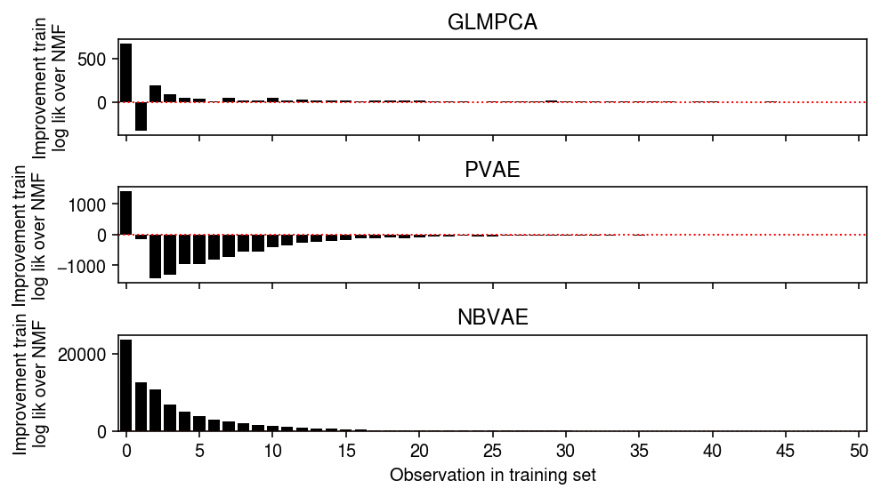
Look at the total training log likelihood differences, stratified by observed value.
plt.clf()
fig, ax = plt.subplots(3, 1, sharex=True)
fig.set_size_inches(7, 4)

grid = np.arange(train.max() + 1)
ax[0].bar(grid, np.array([(llik1 - llik0)[train == i].sum() for i in grid]), color='k')
ax[0].axhline(y=0, ls=':', lw=1, c='r')
ax[0].set_ylabel('Improvement train\nlog lik over NMF')
ax[0].set_title('GLMPCA')

ax[1].bar(grid, np.array([(llik2 - llik0)[train == i].sum() for i in grid]), color='k')
ax[1].axhline(y=0, ls=':', lw=1, c='r')
ax[1].set_ylabel('Improvement train\nlog lik over NMF')
ax[1].set_title('PVAE')

ax[2].bar(grid, np.array([(llik3 - llik0)[train == i].sum() for i in grid]), color='k')
ax[2].axhline(y=0, ls=':', lw=1, c='r')
ax[2].set_ylabel('Improvement train\nlog lik over NMF')
ax[2].set_title('NBVAE')
ax[2].set_xticks(grid[::5])
ax[2].set_xticklabels(grid[::5].astype(int))
ax[2].set_xlim(-.5, grid.max() - .5)
ax[2].set_xlabel('Observation in training set')

fig.tight_layout()
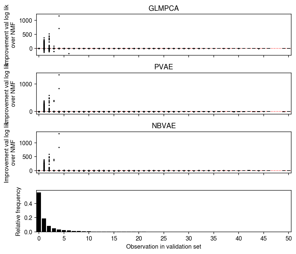
Repeat the analysis for the validation data.
s = (test.sum(axis=1) / train.sum(axis=1)).reshape(-1, 1)
llik0 = st.poisson(s * lam0).logpmf(test)
llik1 = st.poisson(s * lam1).logpmf(test)
llik2 = st.poisson(s * lam2).logpmf(test)
llik3 = st.poisson(s * lam3).logpmf(test)
pd.Series({'NMF': llik0.mean(), 'GLMPCA': llik1.mean(), 'PVAE': llik2.mean(), 'NBVAE': llik3.mean()})
NMF      -1.132348
GLMPCA   -1.087027
PVAE     -1.071313
NBVAE    -1.129745
dtype: float64
plt.clf()
fig, ax = plt.subplots(4, 1, sharex=True)
fig.set_size_inches(7, 6)

grid = np.arange(test.max())
for i in grid:
  ax[0].boxplot((llik1 - llik0)[test == i].ravel(), positions=[i], widths=[0.5], medianprops={'color': 'k'}, flierprops={'marker': '.', 'markersize': 2})
ax[0].axhline(y=0, ls=':', lw=1, c='r')
ax[0].set_ylabel('Improvement val log lik\nover NMF')
ax[0].set_title('GLMPCA')

for i in grid:
  ax[1].boxplot((llik2 - llik0)[test == i].ravel(), positions=[i], widths=[0.5], medianprops={'color': 'k'}, flierprops={'marker': '.', 'markersize': 2})
ax[1].axhline(y=0, ls=':', lw=1, c='r')
ax[1].set_ylabel('Improvement val log lik\nover NMF')
ax[1].set_title('PVAE')

for i in grid:
  ax[2].boxplot((llik3 - llik0)[test == i].ravel(), positions=[i], widths=[0.5], medianprops={'color': 'k'}, flierprops={'marker': '.', 'markersize': 2})
ax[2].axhline(y=0, ls=':', lw=1, c='r')
ax[2].set_ylabel('Improvement val log lik\nover NMF')
ax[2].set_title('NBVAE')

h, e = np.histogram(test.ravel(), bins=np.arange(test.max() + 1), density=True)
ax[3].bar(e[:-1], h, color='k')
ax[3].set_ylabel('Relative frequency')
ax[3].set_xticks(grid[::5])
ax[3].set_xticklabels(grid[::5].astype(int))
ax[3].set_xlim(-.5, grid.max() - .5)
ax[3].set_xlabel('Observation in validation set')

fig.tight_layout()
plt.clf()
fig, ax = plt.subplots(3, 1, sharex=True)
fig.set_size_inches(7, 4)

grid = np.arange(test.max() + 1)
ax[0].bar(grid, np.array([(llik1 - llik0)[test == i].sum() for i in grid]), color='k')
ax[0].axhline(y=0, ls=':', lw=1, c='r', zorder=-3)
ax[0].set_ylabel('Improvement val log lik\nover NMF')
ax[0].set_title('GLMPCA')

ax[1].bar(grid, np.array([(llik2 - llik0)[test == i].sum() for i in grid]), color='k')
ax[1].axhline(y=0, ls=':', lw=1, c='r', zorder=-3)
ax[1].set_ylabel('Improvement val log lik\nover NMF')
ax[1].set_title('PVAE')

ax[2].bar(grid, np.array([(llik3 - llik0)[test == i].sum() for i in grid]), color='k')
ax[2].axhline(y=0, ls=':', lw=1, c='r', zorder=-3)
ax[2].set_ylabel('Improvement val log lik\nover NMF')
ax[2].set_title('NBPVAE')
ax[2].set_xticks(grid[::5])
ax[2].set_xticklabels(grid[::5].astype(int))
ax[2].set_xlim(-.5, grid.max() - .5)
ax[2].set_xlabel('Observation in validation set')

fig.tight_layout()

Count the fraction of observations equal to one in the validation set.
(test == 1).sum() / np.prod(test.shape)
0.187488
For observations which were equal to one in validation set, look at the distribution of training set values.
pd.Series(dict(enumerate([np.logical_and(train == i, test == 1).sum() / (test == 1).sum() for i in range(4)])))
0    0.540323
1    0.254025
2    0.107712
3    0.050151
dtype: float64
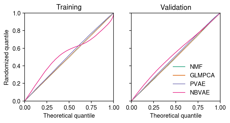
Look at the distribution of (a random sample of) randomized quantiles for each method.
train_qs = []
test_qs = []
for l in [lam0, lam1, lam2]:
  F = st.poisson(l)
  q = np.sort((F.cdf(train - 1) + np.random.uniform(size=train.shape) * F.pmf(train)).ravel()[::10])
  train_qs.append(q)
  q = np.sort((F.cdf(test - 1) + np.random.uniform(size=test.shape) * F.pmf(test)).ravel()[::10])
  test_qs.append(q)
for l in [lam3]:
  F = st.nbinom(n=np.exp(nbvae_log_inv_disp), p=1 / (1 + l * np.exp(-nbvae_log_inv_disp)))
  q = np.sort((F.cdf(train - 1) + np.random.uniform(size=train.shape) * F.pmf(train)).ravel()[::10])
  train_qs.append(q)
  q = np.sort((F.cdf(test - 1) + np.random.uniform(size=test.shape) * F.pmf(test)).ravel()[::10])
  test_qs.append(q)
cm = plt.get_cmap('Dark2')
plt.clf()
fig, ax = plt.subplots(1, 2, sharey=True)
fig.set_size_inches(5.5, 3)
lim = [0, 1]
for a, qs, t in zip(ax.ravel(), [train_qs, test_qs], ['Training', 'Validation']):
  for i, (q, k) in enumerate(zip(qs, ['NMF', 'GLMPCA', 'PVAE', 'NBVAE'])):
    x = np.linspace(0, 1, q.shape[0] + 1)[1:]
    a.plot(x, np.sort(q), lw=1, c=cm(i), label=k)
    a.plot(lim, lim, lw=1, ls=':', c='0.7')
  a.set_xlim(lim)
  a.set_ylim(lim)
  a.set_xlabel('Theoretical quantile')
  a.set_title(t)
ax[0].set_ylabel('Randomized quantile')
ax[1].legend(frameon=False)
fig.tight_layout()
T cell/B cell
Split the data into training and validation sets using binomial thinning, then fit NMF, GLMPCA, and PVAE.
# Important: this implicitly sets the random seed
x = data['cytotoxic_t-b_cells']()
train, test = scmodes.benchmark.train_test_split(x)
np.save('/scratch/midway2/aksarkar/modes/fitted-values/cytotoxic_t-b_cells-train', train)
np.save('/scratch/midway2/aksarkar/modes/fitted-values/cytotoxic_t-b_cells-test', test)
sbatch --partition=broadwl -n1 --mem=8G --time=24:00:00
#!/bin/bash
source activate scmodes
python <<EOF
<<imports>>
train = np.load('/scratch/midway2/aksarkar/modes/fitted-values/cytotoxic_t-b_cells-train.npy')
l, f, _ = scmodes.lra.nmf(train, rank=8, tol=1e-2, max_iters=100000, verbose=True)
lam0 = l @ f.T
np.save('/scratch/midway2/aksarkar/modes/fitted-values/cytotoxic_t-b_cells-nmf-lam', lam0)

l, f, _ = scmodes.lra.glmpca(train, rank=8, tol=1e-2, max_iters=100000, verbose=True)
lam1 = np.exp(l @ f.T)
np.save('/scratch/midway2/aksarkar/modes/fitted-values/cytotoxic_t-b_cells-glmpca-lam', lam1)
EOF
sbatch --partition=gpu2 --gres=gpu:1 --mem=8G
#!/bin/bash
source activate scmodes
python <<EOF
<<imports>>
train = np.load('/scratch/midway2/aksarkar/modes/fitted-values/cytotoxic_t-b_cells-train.npy')
xt = torch.tensor(train, dtype=torch.float)
m = scmodes.lra.PVAE(input_dim=train.shape[1], latent_dim=8).fit(xt, test_size=0.1, lr=1e-3, max_epochs=200, trace=True)
lam2 = m.denoise(xt, n_samples=100)
np.save('/scratch/midway2/aksarkar/modes/fitted-values/cytotoxic_t-b_cells-pvae-lam', lam2)
np.save('/scratch/midway2/aksarkar/modes/fitted-values/cytotoxic_t-b_cells-pvae-trace', np.array(m.trace))
EOF
Read the results.
train = np.load('/scratch/midway2/aksarkar/modes/fitted-values/cytotoxic_t-b_cells-train.npy')
test = np.load('/scratch/midway2/aksarkar/modes/fitted-values/cytotoxic_t-b_cells-test.npy')
lam0 = np.load('/scratch/midway2/aksarkar/modes/fitted-values/cytotoxic_t-b_cells-nmf-lam.npy')
lam1 = np.load('/scratch/midway2/aksarkar/modes/fitted-values/cytotoxic_t-b_cells-glmpca-lam.npy')
lam2 = np.load('/scratch/midway2/aksarkar/modes/fitted-values/cytotoxic_t-b_cells-pvae-lam.npy')
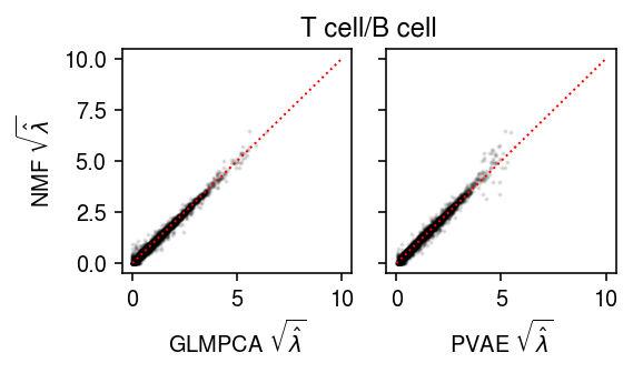
Plot the results.
plt.clf()
fig, ax = plt.subplots(1, 2, sharey=True)
fig.set_size_inches(4, 2.5)

ax[0].scatter(np.sqrt(lam1.ravel()[::50]), np.sqrt(lam0.ravel()[::50]), s=1, c='k', alpha=0.1)
ax[0].plot([0, 10], [0, 10], lw=1, ls=':', c='r')
ax[0].set_xlabel(r'GLMPCA $\sqrt{\hat\lambda}$')
ax[0].set_ylabel(r'NMF $\sqrt{\hat\lambda}$')

ax[1].scatter(np.sqrt(lam2.ravel()[::50]), np.sqrt(lam0.ravel()[::50]), s=1, c='k', alpha=0.1)
ax[1].plot([0, 10], [0, 10], lw=1, ls=':', c='r')
ax[1].set_xlabel(r'PVAE $\sqrt{\hat\lambda}$')

a = fig.add_subplot(111, frame_on=False, xticks=[], yticks=[])
a.set_title('T cell/B cell')
fig.tight_layout()
PBMC
Split the data into training and validation sets using binomial thinning, then fit NMF, GLMPCA, and PVAE.
# Important: this implicitly sets the random seed
x = data['pbmc_10k_v3']()
train, test = scmodes.benchmark.train_test_split(x)
np.save('/scratch/midway2/aksarkar/modes/fitted-values/pbmcs_10k_v3-train', train)
np.save('/scratch/midway2/aksarkar/modes/fitted-values/pbmcs_10k_v3-test', test)
sbatch --partition=broadwl -n1 --mem=8G --time=24:00:00
#!/bin/bash
source activate scmodes
python <<EOF
<<imports>>
train = np.load('/scratch/midway2/aksarkar/modes/fitted-values/pbmcs_10k_v3-train.npy')
l, f, _ = scmodes.lra.nmf(train, rank=8, tol=1e-2, max_iters=100000, verbose=True)
lam0 = l @ f.T
np.save('/scratch/midway2/aksarkar/modes/fitted-values/pbmcs_10k_v3-nmf-lam', lam0)

l, f, _ = scmodes.lra.glmpca(train, rank=8, tol=1e-2, max_iters=100000, verbose=True)
lam1 = np.exp(l @ f.T)
np.save('/scratch/midway2/aksarkar/modes/fitted-values/pbmcs_10k_v3-glmpca-lam', lam1)
EOF
sbatch --partition=gpu2 --gres=gpu:1 --mem=8G
#!/bin/bash
source activate scmodes
python <<EOF
<<imports>>
train = np.load('/scratch/midway2/aksarkar/modes/fitted-values/pbmcs_10k_v3-train.npy')
xt = torch.tensor(train, dtype=torch.float)
m = scmodes.lra.PVAE(input_dim=train.shape[1], latent_dim=8).fit(xt, test_size=0.1, lr=1e-3, max_epochs=200, trace=True)
lam2 = m.denoise(xt, n_samples=100)
np.save('/scratch/midway2/aksarkar/modes/fitted-values/pbmcs_10k_v3-pvae-lam', lam2)
np.save('/scratch/midway2/aksarkar/modes/fitted-values/pbmcs_10k_v3-pvae-trace', np.array(m.trace))
EOF
Read the results.
train = np.load('/scratch/midway2/aksarkar/modes/fitted-values/pbmcs_10k_v3-train.npy')
test = np.load('/scratch/midway2/aksarkar/modes/fitted-values/pbmcs_10k_v3-test.npy')
lam0 = np.load('/scratch/midway2/aksarkar/modes/fitted-values/pbmcs_10k_v3-nmf-lam.npy')
lam1 = np.load('/scratch/midway2/aksarkar/modes/fitted-values/pbmcs_10k_v3-glmpca-lam.npy')
lam2 = np.load('/scratch/midway2/aksarkar/modes/fitted-values/pbmcs_10k_v3-pvae-lam.npy')
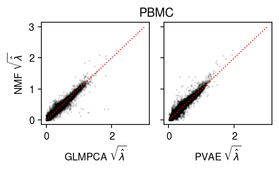
Plot the results.
lim = [0, 3]
plt.clf()
fig, ax = plt.subplots(1, 2, sharey=True)
fig.set_size_inches(4, 2.5)

ax[0].scatter(np.sqrt(lam1.ravel()[::50]), np.sqrt(lam0.ravel()[::50]), s=1, c='k', alpha=0.1)
ax[0].plot(lim, lim, lw=1, ls=':', c='r')
ax[0].set_xlabel(r'GLMPCA $\sqrt{\hat\lambda}$')
ax[0].set_ylabel(r'NMF $\sqrt{\hat\lambda}$')

ax[1].scatter(np.sqrt(lam2.ravel()[::50]), np.sqrt(lam0.ravel()[::50]), s=1, c='k', alpha=0.1)
ax[1].plot(lim, lim, lw=1, ls=':', c='r')
ax[1].set_xlabel(r'PVAE $\sqrt{\hat\lambda}$')

a = fig.add_subplot(111, frame_on=False, xticks=[], yticks=[])
a.set_title('PBMC')
fig.tight_layout()
Liver
Split the data into training and validation sets using binomial thinning, then fit NMF, GLMPCA, and PVAE.
# Important: this implicitly sets the random seed
x = data['liver-caudate-lobe']()
train, test = scmodes.benchmark.train_test_split(x)
np.save('/scratch/midway2/aksarkar/modes/fitted-values/liver-caudate-lobe-train', train)
np.save('/scratch/midway2/aksarkar/modes/fitted-values/liver-caudate-lobe-test', test)
sbatch --partition=broadwl -n1 --mem=8G --time=2:00:00
#!/bin/bash
source activate scmodes
python <<EOF
<<imports>>
train = np.load('/scratch/midway2/aksarkar/modes/fitted-values/liver-caudate-lobe-train.npy')
l, f, _ = scmodes.lra.nmf(train, rank=8, tol=1e-2, max_iters=100000, verbose=True)
lam0 = l @ f.T
np.save('/scratch/midway2/aksarkar/modes/fitted-values/liver-caudate-lobe-nmf-lam', lam0)

l, f, _ = scmodes.lra.glmpca(train, rank=8, tol=1e-2, max_iters=100000, verbose=True)
lam1 = np.exp(l @ f.T)
np.save('/scratch/midway2/aksarkar/modes/fitted-values/liver-caudate-lobe-glmpca-lam', lam1)
EOF
sbatch --partition=gpu2 --gres=gpu:1 --mem=8G
#!/bin/bash
source activate scmodes
python <<EOF
<<imports>>
train = np.load('/scratch/midway2/aksarkar/modes/fitted-values/liver-caudate-lobe-train.npy')
torch.manual_seed(1)
xt = torch.tensor(train, dtype=torch.float)
m = scmodes.lra.PVAE(input_dim=train.shape[1], latent_dim=8).fit(xt, test_size=0.1, lr=1e-3, max_epochs=1600, trace=True)
lam2 = m.denoise(xt, n_samples=100)
np.save('/scratch/midway2/aksarkar/modes/fitted-values/liver-caudate-lobe-pvae-lam', lam2)
np.save('/scratch/midway2/aksarkar/modes/fitted-values/liver-caudate-lobe-pvae-trace', np.array(m.trace))
EOF
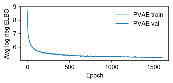
Examine the VAE optimization traces.
cm = plt.get_cmap('Paired')
plt.clf()
plt.gcf().set_size_inches(4, 2)
trace = np.load('/scratch/midway2/aksarkar/modes/fitted-values/liver-caudate-lobe-pvae-trace.npy')
for i, (t, s, k) in enumerate(zip(trace.T, [900, 100], ['PVAE train', 'PVAE val'])):
  plt.plot(np.log(t / s), lw=1, c=cm(i), label=k)
plt.legend(frameon=False)
plt.xlabel('Epoch')
plt.ylabel('Avg log neg ELBO')
plt.tight_layout()
Read the results.
train = np.load('/scratch/midway2/aksarkar/modes/fitted-values/liver-caudate-lobe-train.npy')
test = np.load('/scratch/midway2/aksarkar/modes/fitted-values/liver-caudate-lobe-test.npy')
lam0 = np.load('/scratch/midway2/aksarkar/modes/fitted-values/liver-caudate-lobe-nmf-lam.npy')
lam1 = np.load('/scratch/midway2/aksarkar/modes/fitted-values/liver-caudate-lobe-glmpca-lam.npy')
lam2 = np.load('/scratch/midway2/aksarkar/modes/fitted-values/liver-caudate-lobe-pvae-lam.npy')
s = (test.sum(axis=1) / train.sum(axis=1)).reshape(-1, 1)
llik0 = st.poisson(s * lam0).logpmf(test)
llik1 = st.poisson(s * lam1).logpmf(test)
llik2 = st.poisson(s * lam2).logpmf(test)
pd.Series({'NMF': llik0.mean(), 'GLMPCA': llik1.mean(), 'PVAE': llik2.mean()})
NMF      -0.961543
GLMPCA   -0.940434
PVAE     -0.979979
dtype: float64
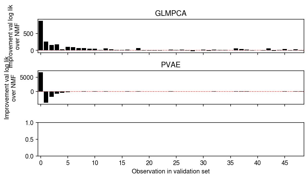
Plot the results.
plt.clf()
fig, ax = plt.subplots(3, 1, sharex=True)
fig.set_size_inches(7, 4)

grid = np.arange(50)
ax[0].bar(grid, np.array([(llik1 - llik0)[test == i].sum() for i in grid]), color='k')
ax[0].axhline(y=0, ls=':', lw=1, c='r', zorder=-3)
ax[0].set_ylabel('Improvement val log lik\nover NMF')
ax[0].set_title('GLMPCA')

ax[1].bar(grid, np.array([(llik2 - llik0)[test == i].sum() for i in grid]), color='k')
ax[1].axhline(y=0, ls=':', lw=1, c='r', zorder=-3)
ax[1].set_ylabel('Improvement val log lik\nover NMF')
ax[1].set_title('PVAE')

ax[-1].set_xticks(grid[::5])
ax[-1].set_xticklabels(grid[::5].astype(int))
ax[-1].set_xlim(-.5, grid.max() - .5)
ax[-1].set_xlabel('Observation in validation set')

fig.tight_layout()
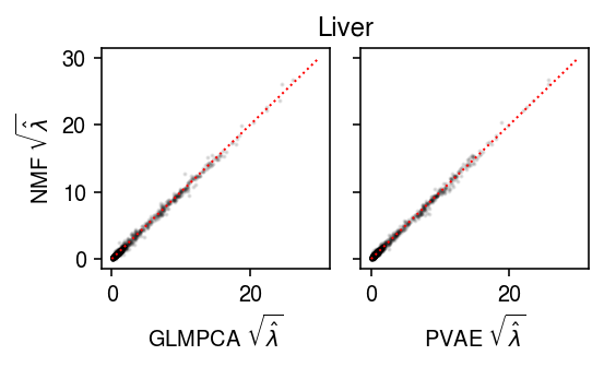
lim = [0, 30]
plt.clf()
fig, ax = plt.subplots(1, 2, sharey=True)
fig.set_size_inches(4, 2.5)

ax[0].scatter(np.sqrt(lam1.ravel()[::50]), np.sqrt(lam0.ravel()[::50]), s=1, c='k', alpha=0.1)
ax[0].plot(lim, lim, lw=1, ls=':', c='r')
ax[0].set_xlabel(r'GLMPCA $\sqrt{\hat\lambda}$')
ax[0].set_ylabel(r'NMF $\sqrt{\hat\lambda}$')

ax[1].scatter(np.sqrt(lam2.ravel()[::50]), np.sqrt(lam0.ravel()[::50]), s=1, c='k', alpha=0.1)
ax[1].plot(lim, lim, lw=1, ls=':', c='r')
ax[1].set_xlabel(r'PVAE $\sqrt{\hat\lambda}$')

a = fig.add_subplot(111, frame_on=False, xticks=[], yticks=[])
a.set_title('Liver')
fig.tight_layout()