Speed up ash mode estimation

Introduction
Setup
Results

Introduction

We want to deconvolve scRNA-seq data assuming \(g_j\) is some unimodal distribution over non-negative reals. In practice, we represent this family of distribution as

\[ g_j = \sum_{k=1}^K \pi_k \mathrm{Uniform}(\cdot; \lambda_0, a_{jk}) \]

where \(K\) is sufficiently large and \(\lambda_0\) is the mode (Stephens 2016).

To estimate the mode \(\lambda_{0j}\) for gene \(j\), we find:

\[ \lambda_{0j}^* = \arg\max_{\lambda_{0j}} \sum_i \int f(x_i \mid \lambda_i) g_j(\lambda_i \mid \pi, \lambda_{0j})\ d\lambda_i \]

using golden section search. Here, we investigate practical issues in this approach.

Setup

import functools as ft
import multiprocessing as mp
import numpy as np
import pandas as pd
import scipy.stats as st
import scipy.special as sp
import scmodes
import scqtl
import sklearn.model_selection as skms

import rpy2.robjects.packages
import rpy2.robjects.pandas2ri
import rpy2.robjects.numpy2ri

rpy2.robjects.pandas2ri.activate()
rpy2.robjects.numpy2ri.activate()

ashr = rpy2.robjects.packages.importr('ashr')
descend = rpy2.robjects.packages.importr('descend')

%matplotlib inline
%config InlineBackend.figure_formats = set(['retina'])

import colorcet
import matplotlib.pyplot as plt
plt.rcParams['figure.facecolor'] = 'w'
plt.rcParams['font.family'] = 'Nimbus Sans'

Results

Convexity

As an example, use the highest expressed genes in 10K sorted CD8+ cytotoxic T cells Zheng et al. 2017.

x = scmodes.dataset.read_10x('/project2/mstephens/aksarkar/projects/singlecell-ideas/data/10xgenomics/cytotoxic_t/filtered_matrices_mex/hg19')
xj = pd.Series(x[:,x.mean(axis=0).argmax()])
size_factor = pd.Series(x.sum(axis=1))
lam = xj / size_factor

Mengyin Liu claimed this problem is convex in \(\lambda_{0j}\), However, on the above example, the quality of the result depends on the bounds of the search. Is this problem actually convex?

By default, the bounds are \([\min(x_i), \max(x_i)]\), which can be extremely large. However, we need to remove the scaling factor, so should we instead search over \([\min(x_i / R_i), \max(x_i / R_i)]\)? The motivation for the proposed alternative is to only look over plausible values of \(\lambda_i\).

grid = np.geomspace(1e-3, xj.max(), 100)
llik = np.array([np.array(
  ashr.ash(
    pd.Series(np.zeros(xj.shape)),
    1,
    lik=ashr.lik_pois(y=xj, scale=size_factor, link='identity'),
    mode=lam0,
    outputlevel='loglik').rx2('loglik')) for lam0 in grid]).ravel()

res0 = ashr.ash(
  pd.Series(np.zeros(xj.shape)),
  1,
  lik=ashr.lik_pois(y=xj, scale=size_factor, link='identity'),
  mode='estimate')
res1 = ashr.ash(
  pd.Series(np.zeros(x.shape[0])),
  1,
  lik=ashr.lik_pois(y=xj, scale=size_factor, link='identity'),
  mode=pd.Series([lam.min(), lam.max()]))

plt.clf()
plt.gcf().set_size_inches(3, 3)
plt.xscale('log')
plt.plot(grid, np.array(llik).ravel(), lw=1, c='k')
plt.axvline(x=np.array(res0.rx2('fitted_g').rx2('a'))[0], c='k', lw=1, ls=':', label='Default')
plt.axvline(x=np.array(res1.rx2('fitted_g').rx2('a'))[0], c='r', lw=1, ls=':', label='Restricted')
plt.legend(frameon=False, loc='center left', bbox_to_anchor=(1, .5))
plt.xlabel('Mode $\lambda_0$')
_ = plt.ylabel('Marginal likelihood')

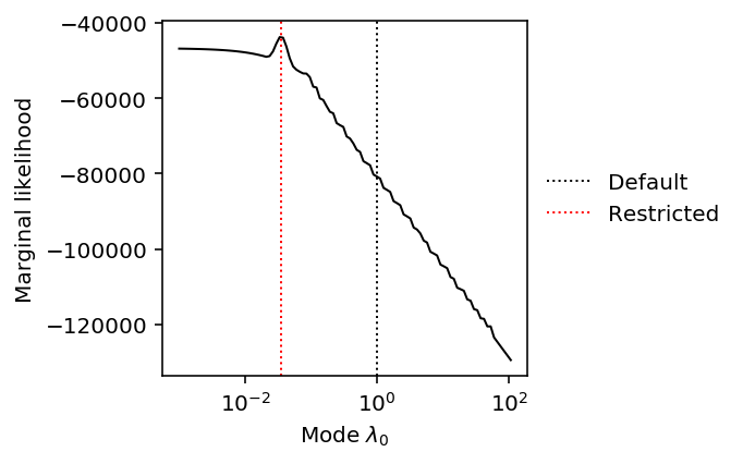
It appears the problem is actually non-convex. Surprisingly, it appears non-convex even for a case where the data are not bimodal. For bimodal data, we might expect that choice of the mode would change the weight on/near zero and result in a non-convex objective.

According to the documentation, the search can fail for poor choice of initial query, which depends entirely on the initial interval. In this example, the initial interval does not contain the mode, and therefore the search finds the correct local optimum within the interval, but fails to find the global optimum.

This result does not necessarily mean that our proposed alternative, to search over \([\min(x_i / R_i), \max(x_i / R_i)]\) will work, because Poisson noise could mean the true \(\lambda_i > x_i / R_i\) for some sample \(i\).

Should we search further to be reasonably certain we haven't missed the mode? Intuitively, the largest \(\hat\lambda_i\) value we do observe should be "overestimated"; if it were not, then we should expect higher density of \(g\) around it, and values larger than it in the observed data.

Speed

We have to solve an ash subproblem for each query \(\lambda_0\), which becomes extremely expensive for large data sets. We can speed up the procedure by downsampling the data for mode estimation. How much worse is the fitted model?

def score_mode_estimation(data, seed=0, p=0.1):
  temp = data.sample(random_state=seed, frac=p)
  res0 = ashr.ash(
    pd.Series(np.zeros(temp.shape[0])),
    1,
    lik=ashr.lik_pois(y=temp['x'], scale=temp['scale'], link='identity'),
    mode=pd.Series([temp['lam'].min(), temp['lam'].max()]))
  lam0 = np.array(res0.rx2('fitted_g').rx2('a'))[0]
  res = ashr.ash(
    pd.Series(np.zeros(data.shape[0])),
    1,
    lik=ashr.lik_pois(y=data['x'], scale=data['scale'], link='identity'),
    mode=lam0)
  return lam0, np.array(res.rx2('loglik'))[0]

def evaluate_mode_estimation(data, num_trials):
  result = []
  for p in (0.1, 0.25, 0.5):
    for trial in range(num_trials):
      lam0, llik = score_mode_estimation(data, seed=trial, p=p)
      result.append([p, trial, lam0, llik])
  result = pd.DataFrame(result, columns=['p', 'trial', 'lam0', 'llik'])
  return result

mode_estimation_result = evaluate_mode_estimation(pd.DataFrame({'x': xj, 'scale': size_factor, 'lam': lam}), num_trials=10)

plt.clf()
plt.gcf().set_size_inches(3, 3)
plt.scatter(mode_estimation_result['p'], mode_estimation_result['llik'], s=4, c='k')
plt.axhline(y=np.array(res1.rx2('loglik'))[0], c='k', lw=1, ls=':')
plt.xlabel('Fraction of original data')
plt.ylabel('Training log likelihood')

Text(0, 0.5, 'Training log likelihood')

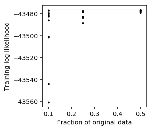
Downsampling is likely to result in a much worse model fit, so we should not pursue that strategy to speed up the model estimation.

Using a simpler model

We previously found an example of near-Poisson data where ash mode estimation fails.

data, _ = scqtl.simulation.simulate(num_samples=1000, logodds=-5, seed=2)
x = pd.Series(data[:,0])
s = pd.Series(data[:,1])
lam = x / s

Plot the data.

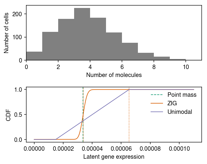
Fit \(g\) assuming a point mass \(\mu\).

fit0 = scqtl.simple.fit_pois(x, s)

Fit \(g\) assuming Gamma.

\[ \lambda_i \sim \operatorname{Gamma}(1/\phi, 1/(\mu\phi)) \]

# Important: this returns mu, 1/phi
fit1 = scqtl.simple.fit_nb(x, s)

Report the estimated modes and log likelihoods.

# Important: Gamma(a, b) mode is max((a - 1) / b, 0)
pd.DataFrame({'mode': [fit0[0], fit1[0] * (fit1[1] - 1) / fit1[1]], 'llik': [fit0[-1], fit1[-1]]}, index=['pointmass', 'gamma'])

mode         llik
pointmass  0.000034 -2008.663140
gamma      0.000033 -2008.503731

The unimodal distribution is parameterized:

\[ g = \sum_{k=1}^{K} w_k \operatorname{Uniform}(\lambda_0, \lambda_0 \pm a_k) \]

where we abuse notation for brevity, and the endpoints \(a_k\) follow a geometric series. Fix the mode to the Gamma mode, and fit unimodal \(g\) for different choices of ratio between successive endpoints.

ratio = np.linspace(1.1, 1.5, 50)
res = []
for r in ratio:
  low = 1 / s.mean()
  high = (x / s).max()
  mixsd = pd.Series(np.exp(np.arange(np.log(low), np.log(high), step=np.log(r))))
  fit = ashr.ash_workhorse(
    pd.Series(np.zeros(x.shape)), 1,
    lik=ashr.lik_pois(y=x, scale=s, link='identity'),
    mixsd=mixsd,
    mode=fit1[0] * (fit1[1] - 1) / fit1[1],
    output=pd.Series(['loglik', 'fitted_g']))
  res.append([r, np.array(fit.rx2('loglik'))[0], np.array(fit.rx2('fitted_g').rx2('pi'))[0]])
res = pd.DataFrame(res)
res.columns = ['ratio', 'llik', 'pi0']

Plot the log likelihood versus chosen ratio. Mark the location of ratio \(\sqrt{2}\).

plt.clf()
plt.gcf().set_size_inches(3, 3)
plt.plot(res['ratio'], res['llik'], lw=1, c='k')
plt.axvline(x=np.sqrt(2), ls=':', c='r', lw=1)
plt.xlabel('Ratio')
plt.ylabel('Log liklihood')
plt.tight_layout()

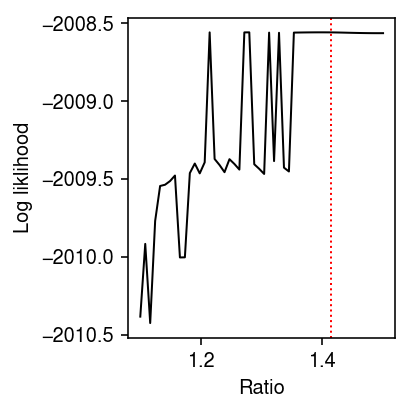
Report the ratio which achieves the best log likelihood.

res.loc[res['pi0'].idxmax()]

ratio       1.434694
llik    -2008.561414
pi0         0.966383
Name: 41, dtype: float64

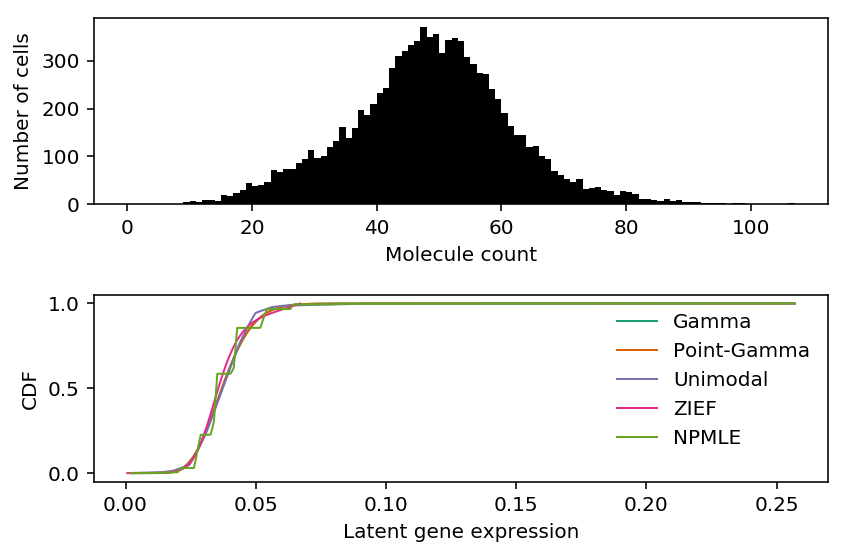
Try applying this approach to the highest expressed genes in 10K sorted CD8+ cytotoxic T cells Zheng et al. 2017.

x = scmodes.dataset.read_10x('/project2/mstephens/aksarkar/projects/singlecell-ideas/data/10xgenomics/cytotoxic_t/filtered_matrices_mex/hg19', return_df=True)
xj = x[x.mean(axis=0).idxmax()]
s = x.sum(axis=1)
lam = xj / s

Fit Gamma, and test for goodness of fit.

init = scqtl.simple.fit_nb(xj, s)
scmodes.benchmark.gof._gof(
  xj.values.ravel(),
  cdf=scmodes.benchmark.gof._zig_cdf,
  pmf=scmodes.benchmark.gof._zig_pmf,
  size=s.values.ravel(),
  log_mu=np.log(init[0]),
  log_phi=-np.log(init[1]))

KstestResult(statistic=0.0186349904442156, pvalue=0.0016661060591321017)

Fit unimodal, and test for goodness of fit.

fit = ashr.ash_workhorse(
  pd.Series(np.zeros(xj.shape)), 1,
  lik=ashr.lik_pois(y=xj, scale=s, link='identity'),
  mixsd=pd.Series(np.exp(np.arange(np.log(1 / s.mean()), np.log((xj / s).max()), step=.5 * np.log(2)))),
  mode=init[0] * (init[1] - 1) / init[1],
  output=pd.Series(['loglik', 'fitted_g', 'data']))
scmodes.benchmark.gof._gof(xj, cdf=scmodes.benchmark.gof._ash_cdf, pmf=scmodes.benchmark.gof._ash_pmf, fit=fit, s=s)

KstestResult(statistic=0.059205028160045026, pvalue=1.6543190838957947e-31)

Previously, we found full mode search worked on this example.

fit_estmode = ashr.ash_workhorse(
  pd.Series(np.zeros(xj.shape)), 1,
  lik=ashr.lik_pois(y=xj, scale=s, link='identity'),
  mixsd=pd.Series(np.exp(np.arange(np.log(1 / s.mean()), np.log((xj / s).max()), step=.5 * np.log(2)))),
  mode=pd.Series([lam.min(), lam.max()]),
  output=pd.Series(['loglik', 'fitted_g', 'data']))
scmodes.benchmark.gof._gof(xj, cdf=scmodes.benchmark.gof._ash_cdf, pmf=scmodes.benchmark.gof._ash_pmf, fit=fit_estmode, s=s)

KstestResult(statistic=0.02630989797207417, pvalue=1.4551355049273953e-06)

Report the estimated modes and marginal log likelihood of the fits.

pd.DataFrame(
  {
    'mode': [init[0] * (init[1] - 1) / init[1], init[0] * (init[1] - 1) / init[1], np.array(fit_estmode.rx2('fitted_g').rx2('a'))[0]],
    'llik': [init[-1], np.array(fit.rx2('loglik'))[0], np.array(fit_estmode.rx2('loglik'))[0]]
  },
  index=['gamma', 'unimodal_gamma', 'unimodal'])

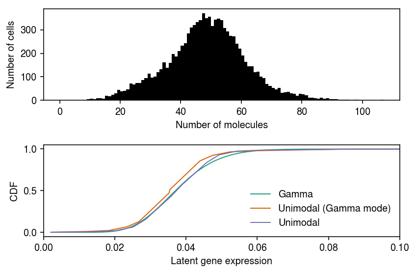
mode          llik
gamma           0.035399 -41349.739021
unimodal_gamma  0.035399 -41409.282482
unimodal        0.037238 -41274.359548

Plot the data, and the fitted distributions.

grid = pd.Series(np.linspace(lam.min(), lam.max(), 1000))
gamma_cdf = st.gamma(a=init[1], scale=init[0] / init[1]).cdf(grid)
unimodal_cdf = np.array(ashr.cdf_ash(fit, grid).rx2('y')).ravel()
estmode_cdf = np.array(ashr.cdf_ash(fit_estmode, grid).rx2('y')).ravel()

cm = plt.get_cmap('Dark2')
plt.clf()
fig, ax = plt.subplots(2, 1)
fig.set_size_inches(6, 4)
ax[0].hist(xj.values, bins=np.arange(xj.values.max() + 1), color='k')
ax[0].set_xlabel('Number of molecules')
ax[0].set_ylabel('Number of cells')

for i, (k, F) in enumerate(zip(['Gamma', 'Unimodal (Gamma mode)', 'Unimodal'], [gamma_cdf, unimodal_cdf, estmode_cdf])):
  ax[1].plot(grid, F, c=cm(i), label=k, lw=1)
ax[1].set_xlim(0, 0.1)
ax[1].legend(frameon=False)
ax[1].set_xlabel('Latent gene expression')
ax[1].set_ylabel('CDF')

fig.tight_layout()

Try denser grids, and report the log likelihoods.

pd.Series({step: np.array(ashr.ash_workhorse(
  pd.Series(np.zeros(xj.shape)), 1,
  lik=ashr.lik_pois(y=xj, scale=s, link='identity'),
  mixsd=pd.Series(np.exp(np.arange(np.log(1 / s.mean()), np.log((xj / s).max()), step=np.log(step)))),
  mode=pd.Series([lam.min(), lam.max()]),
  output=pd.Series(['loglik'])).rx2('loglik'))[0]
              for step in (1.1, 1.15, 1.2, 1.25, 1.3)})

1.10   -41273.537196
1.15   -41273.525195
1.20   -41273.574435
1.25   -41273.954289
1.30   -41273.725401
dtype: float64