Deconvolution of near-Poisson data
Table of Contents
Introduction
Deconvolution of Poisson data assuming a point mass is trivial:
\begin{align*} x_i &\sim \operatorname{Poisson}(s_i \lambda_i)\\ \lambda_i &\sim \delta_\mu(\cdot)\\ \hat\mu &= \frac{\sum_i x_i}{\sum_i s_i} \end{align*}More general approaches should all be able to fit this case. Here, we investigate cases where they fail.
Setup
import numpy as np
import pandas as pd
import scipy.special as sp
import scipy.stats as st
import scmodes
import scqtl.simple

import rpy2.robjects.packages
import rpy2.robjects.pandas2ri

rpy2.robjects.pandas2ri.activate()

ashr = rpy2.robjects.packages.importr('ashr')
descend = rpy2.robjects.packages.importr('descend')
%matplotlib inline
%config InlineBackend.figure_formats = set(['retina'])
import matplotlib.pyplot as plt
plt.rcParams['figure.facecolor'] = 'w'
plt.rcParams['font.family'] = 'Nimbus Sans'
Results
Extract the examples.
Read the results of benchmarking deconvolution methods on homogeneous tissues.
benchmark = {}
for data in ('cytotoxic_t', 'b_cells', 'ipsc'):
  benchmark[data] = (
    pd.read_csv(f'/project2/mstephens/aksarkar/projects/singlecell-modes/data/deconv-generalization/{data}-gpu.txt.gz', index_col=0, sep='\t')
    .merge(pd.read_csv(f'/project2/mstephens/aksarkar/projects/singlecell-modes/data/deconv-generalization/{data}-unimodal.txt.gz', index_col=0, sep='\t'), left_index=True, right_index=True)
    .merge(pd.read_csv(f'/project2/mstephens/aksarkar/projects/singlecell-modes/data/deconv-generalization/{data}-zief.txt.gz', index_col=0, sep='\t'), left_index=True, right_index=True)
    .merge(pd.read_csv(f'/project2/mstephens/aksarkar/projects/singlecell-modes/data/deconv-generalization/{data}-npmle.txt.gz', index_col=0, sep='\t'), left_index=True, right_index=True))
Extract the genes for which ZIEF does best.
query = benchmark['b_cells'][benchmark['b_cells']['zief'] > benchmark['b_cells']['gamma']].index
Read the count matrix.
b_cells = scmodes.dataset.read_10x('/project2/mstephens/aksarkar/projects/singlecell-ideas/data/10xgenomics/b_cells/filtered_matrices_mex/hg19/', return_df=True)
s = b_cells.sum(axis=1)
Read the gene metadata.
gene_info = pd.read_csv('/project2/mstephens/aksarkar/projects/singlecell-qtl/data/scqtl-genes.txt.gz', sep='\t', index_col=0)
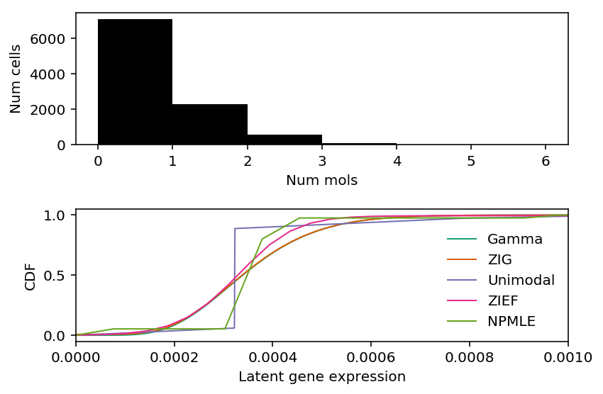
Deconvolve specific examples
Fit various deconvolutions.
x = b_cells.loc[:,query[0]]
lam = x / s
K = 100
grid = np.linspace(0, lam.max(), K + 1)
gamma_res = scqtl.simple.fit_nb(x, s)
zig_res = scqtl.simple.fit_zinb(x, s)
unimodal_res = ashr.ash_workhorse(
    pd.Series(np.zeros(x.shape)),
    1,
    outputlevel=pd.Series(['fitted_g', 'loglik']),
    lik=ashr.lik_pois(y=x, scale=s, link='identity'),
    mixsd=pd.Series(np.geomspace(lam.min() + 1e-8, lam.max(), 25)),
    mode=pd.Series([lam.min(), lam.max()]))
zief_res = descend.deconvSingle(x, scaling_consts=s, verbose=False)
npmle_res = ashr.ash_workhorse(
    pd.Series(np.zeros(x.shape)),
    1,
    outputlevel=pd.Series(['fitted_g', 'loglik']),
    lik=ashr.lik_pois(y=x, scale=s, link='identity'),
    g=ashr.unimix(pd.Series(np.ones(K) / K), pd.Series(grid[:-1]), pd.Series(grid[1:])))
Discretize the CDFs.
grid = np.linspace(lam.min(), 1e-3, 1000)
gamma_cdf = st.gamma(a=gamma_res[1], scale=gamma_res[0] / gamma_res[1]).cdf(grid)
zig_cdf = gamma_cdf * sp.expit(-zig_res[2]) + sp.expit(zig_res[2])
unimodal_cdf = ashr.cdf_ash(unimodal_res, grid)
zief_g = np.array(zief_res.slots['distribution'])[:,:2]
zief_cdf = np.array([zief_g[:,0], np.cumsum(zief_g[:,1])])
npmle_cdf = ashr.cdf_ash(npmle_res, grid)
plt.clf()
fig, ax = plt.subplots(2, 1)
fig.set_size_inches(6, 4)
ax[0].hist(x, bins=np.arange(x.max() + 1), color='k')
ax[0].set_xlabel('Num mols')
ax[0].set_ylabel('Num cells')

cm = plt.get_cmap('Dark2').colors
ax[1].set_xlim(0, 1e-3)
ax[1].plot(grid, gamma_cdf, color=cm[0], lw=1, label='Gamma')
ax[1].plot(grid, zig_cdf, color=cm[1], lw=1, label='ZIG')
ax[1].plot(np.array(unimodal_cdf.rx2('x')),
           np.array(unimodal_cdf.rx2('y')).ravel(), c=cm[2], lw=1, label='Unimodal')
ax[1].plot(zief_cdf[0], zief_cdf[1], c=cm[3], lw=1, label='ZIEF')
ax[1].plot(np.array(npmle_cdf.rx2('x')),
           np.array(npmle_cdf.rx2('y')).ravel(), c=cm[4], lw=1, label='NPMLE')
ax[1].set_xlabel('Latent gene expression')
ax[1].set_ylabel('CDF')
ax[1].legend(frameon=False)

fig.tight_layout()
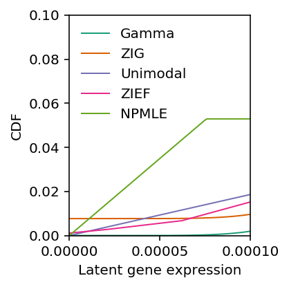
Zoom in around 0.
plt.clf()
plt.gcf().set_size_inches(3, 3)
cm = plt.get_cmap('Dark2').colors
plt.xlim(0, 1e-4)
plt.ylim(0, .1)
plt.xticks([0, 5e-5, 1e-4])
plt.plot(grid, gamma_cdf, color=cm[0], lw=1, label='Gamma')
plt.plot(grid, zig_cdf, color=cm[1], lw=1, label='ZIG')
plt.plot(np.array(unimodal_cdf.rx2('x')),
         np.array(unimodal_cdf.rx2('y')).ravel(), c=cm[2], lw=1, label='Unimodal')
plt.plot(zief_cdf[0], zief_cdf[1], c=cm[3], lw=1, label='ZIEF')
plt.plot(np.array(npmle_cdf.rx2('x')),
         np.array(npmle_cdf.rx2('y')).ravel(), c=cm[4], lw=1, label='NPMLE')
plt.xlabel('Latent gene expression')
plt.ylabel('CDF')
plt.legend(frameon=False)
plt.tight_layout()
Report the training log likelihoods.
point_llik = st.poisson(mu=x.sum() / s.sum()).logpmf(x)
gamma_llik = st.nbinom(n=gamma_res[1], p=1 / (1 + s * gamma_res[0] / gamma_res[1])).logpmf(x)
zig_llik = np.where(x < 1,
                    -np.log1p(np.exp(-zig_res[2])) + np.log1p(np.exp(gamma_llik - zig_res[2])),
                    -np.log1p(np.exp(zig_res[2])) + gamma_llik)
unimodal_llik = np.array(unimodal_res.rx2('loglik'))
zief_llik = np.where(x < 1,
                     np.log(st.poisson(mu=s.values.reshape(-1, 1) * zief_g[:,0]).pmf(x.values.reshape(-1, 1)).dot(zief_g[:,1])),
                     np.log(st.poisson(mu=s.values.reshape(-1, 1) * zief_g[1:,0]).pmf(x.values.reshape(-1, 1)).dot(zief_g[1:,1])))
npmle_llik = np.array(npmle_res.rx2('loglik'))
pd.Series({'Point': point_llik.sum(),
           'Gamma': gamma_llik.sum(),
           'ZIG': zig_llik.sum(),
           'Unimodal': unimodal_llik.sum(),
           'ZIEF': zief_llik.sum(),
           'NPMLE': npmle_llik.sum()})
Point      -31653.253236
Gamma       -7702.696681
ZIG         -7702.818529
Unimodal    -7702.849389
ZIEF        -7702.299609
NPMLE       -7701.940404
dtype: float64
The reason ZIEF appeared anomalous in our benchmark was that our implementation of the validation set log likelihood, marginalizing over the estimated latent distribution \(\hat{g}\), was incorrect.
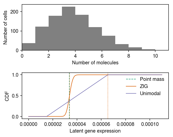
Poisson ash
Draw some near-Poisson data.
data, _ = scqtl.simulation.simulate(num_samples=1000, logodds=-5, seed=2)
x = pd.Series(data[:,0])
s = pd.Series(data[:,1])
lam = x / s
Write out the data.
rpy2.robjects.r['saveRDS'](pd.DataFrame({'x': x, 's': s}), 'pois-mode-est.Rds')
rpy2.rinterface.NULL
Fit Poisson convolved with point mass.
fit0 = scqtl.simple.fit_pois(x, s)
Fit ZINB.
fit1 = scqtl.simple.fit_zinb(x, s)
Fit Poisson ash.
fit2 = ashr.ash_workhorse(
  # these are ignored by ash
  pd.Series(np.zeros(x.shape)),
  1,
  outputlevel=pd.Series(['loglik', 'fitted_g']),
  lik=ashr.lik_pois(y=x, scale=s, link='identity'),
  mixcompdist='halfuniform',
  mixsd=pd.Series(np.geomspace(lam.min() + 1e-8, lam.max(), 25)))
Report the log likelihood.
pd.Series({'pointmass': fit0[-1],
           'zig': fit1[-1],
           'unimodal': np.array(fit2.rx2('loglik'))[0]})
pointmass   -2008.663140
zig         -2008.407921
unimodal    -2077.552567
dtype: float64
Plot the data and estimated \(\hat{g}\). Also plot the estimated mode.
cm = plt.get_cmap('Dark2')
plt.clf()
fig, ax = plt.subplots(2, 1)
fig.set_size_inches(5, 4)
ax[0].hist(x.values, bins=np.arange(x.max() + 1), color='0.5')
ax[0].set_xlim(0, x.max())
ax[0].set_xlabel('Number of molecules')
ax[0].set_ylabel('Number of cells')

ax[1].axvline(x=fit0[0], c=cm(0), lw=1, ls='--', label='Point mass')
ax[1].plot(grid, zinb_cdf, lw=1, c=cm(1), label='ZIG')
ax[1].axvline(x=fit1[0], c=cm(1), ls=':', lw=1)
ax[1].plot(grid, Fx, lw=1, c=cm(2), label='Unimodal')
ax[1].axvline(x=np.array(fit2.rx2('fitted_g').rx2('a'))[0], c=cm(1), ls=':', lw=1)
ax[1].legend(frameon=False)
ax[1].set_xlabel('Latent gene expression')
ax[1].set_ylabel('CDF')

fig.tight_layout()
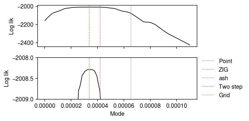
Examine mode estimation.
mode = ashr.ash_estmode(
  betahat=pd.Series(np.zeros(x.shape)),
  sebetahat=1,
  modemin=lam.min(),
  modemax=lam.max(),
  lik=ashr.lik_pois(y=x, scale=s, link='identity'),
  mixcompdist='halfuniform',
  mixsd=pd.Series(np.geomspace(lam.min() + 1e-8, lam.max(), 25)))
mode = np.array(mode)[0]
fit3 = ashr.ash_workhorse(
  # these are ignored by ash
  pd.Series(np.zeros(x.shape)),
  1,
  outputlevel=pd.Series(['loglik', 'fitted_g']),
  lik=ashr.lik_pois(y=x, scale=s, link='identity'),
  mixcompdist='halfuniform',
  mixsd=pd.Series(np.geomspace(lam.min() + 1e-8, lam.max(), 25)),
  mode=mode)
Evaluate the ash log likelihood on a grid of modes, over the space that
ash.estmode optimizes over.
grid = np.linspace(lam.min(), lam.max(), 1000)[1:]
llik = []
for l in grid:
  fit = ashr.ash_workhorse(
         # these are ignored by ash
         pd.Series(np.zeros(x.shape)),
         1,
         outputlevel=pd.Series(['loglik']),
         lik=ashr.lik_pois(y=x, scale=s, link='identity'),
         mixcompdist='halfuniform',
         mixsd=pd.Series(np.geomspace(lam.min() + 1e-8, lam.max(), 25)),
         mode=l)
  llik.append(np.array(fit.rx2('loglik'))[0])
llik = np.array(llik)
Plot the marginal likelihood against the mode.
cm = plt.get_cmap('Dark2')
plt.clf()
fig, ax = plt.subplots(2, 1, sharex=True)
fig.set_size_inches(6, 3)
for a in ax:
  a.plot(grid, llik, lw=1, c='k')
  for i, (m, l) in enumerate(zip([fit0[0], fit1[0], np.array(fit2.rx2('fitted_g').rx2('a'))[0], mode, grid[np.argmax(llik)]], ['Point', 'ZIG', 'ash', 'Two step', 'Grid'])):
    a.axvline(x=m, lw=1, c=cm(i), ls=':', label=l)

ax[1].legend(frameon=False, bbox_to_anchor=(1, .5), loc='center left')
ax[1].set_xlabel('Mode')
ax[1].set_ylim(-2009, -2008)
for a in ax:
  a.set_ylabel('Log lik')
fig.tight_layout()
Report the log likelihood of the two step approach.
pd.Series({'pointmass': fit0[-1],
           'zig': fit1[-1],
           'unimodal': np.array(fit2.rx2('loglik'))[0],
           'twostep': np.array(fit3.rx2('loglik'))[0],
          })
pointmass   -2008.663140
zig         -2008.407921
unimodal    -2077.552567
twostep     -2008.891981
dtype: float64