Differential variance analysis

Introduction
Setup
Methods
Results

Introduction

We previously hypothesized that QTLs could disrupt the mechanisms controlling the variance of gene expression, and therefore reveal new insights into the genetic regulation of differentiation and disease. To investigate this hypothesis, we directly observed gene expression variance across 53 individuals using scRNA-seq, and sought to identify dispersion QTLs (dQTLs) which could alter the variance of gene expression across cells within a single individual, independently of altering the mean expression. However, we failed to discover such QTLs, and demonstrated that variance QTLs can be explained by effects on mean expression (Sarkar et al. 2019). \( \DeclareMathOperator\Poi{Poisson} \DeclareMathOperator\B{Beta} \DeclareMathOperator\E{E} \DeclareMathOperator\Gam{Gamma} \DeclareMathOperator\KL{\mathcal{KL}} \DeclareMathOperator\N{Normal} \DeclareMathOperator\V{V} \newcommand\delmu{\delta_{\mu}} \newcommand\delphi{\delta_{\phi}} \newcommand\const{\mathrm{const}} \newcommand\kr{k_r} \newcommand\kon{k_{\text{on}}} \newcommand\koff{k_{\text{off}}} \newcommand\vtheta{\boldsymbol{\theta}} \newcommand\vx{\mathbf{x}} \newcommand\vs{\mathbf{s}} \newcommand\vz{\mathbf{z}} \)

Before attempting to map dQTLs in a followup study, we need to produce evidence that there are such effects to find in human cell types. Essentially no studies demonstrate mechanistic evidence of such effects in human tissues. Many studies measure gene expression variance in human tissues without estimating the effect of perturbation (e.g. Raj et al. 2006, Shalek et al. 2013; Shalek et al. 2014). Martinez-Jimenez et al. 2018 (re-analyzed by Eling et al. 2018) showed that aging changes variability of mouse CD4+ cell gene expression; however, clearly this perturbation is a complex combination of environmental factors. (This data was not generated using UMIs, further complicating the analysis.) The strongest evidence is presented by Wills et al. 2013, who demonstrated that perturbation of human naive B lymphocytes with a GSK3 inhibitor leads to changes in variance of downstream gene expression (as measured by qPCR).

Here, we develop a method to test for differential variance, and use existing scRNA-seq datasets to ask whether there are effects which can alter gene expression variance independent of altering mean gene expression.

Setup

import anndata
import itertools as it
import numpy as np
import pandas as pd
import pickle
import poisbeta
import scanpy as sc
import scipy.io as si
import scipy.special as sp
import scipy.stats as st
import scmodes
import sklearn.decomposition as skd
import sqlite3
import torch
import torch.utils.tensorboard as tb

%matplotlib inline
%config InlineBackend.figure_formats = set(['retina'])

import colorcet
import matplotlib.pyplot as plt
plt.rcParams['figure.facecolor'] = 'w'
plt.rcParams['font.family'] = 'Nimbus Sans'

Methods

Mechanistic basis of effects on variance

A simple model for transcriptional regulation is the telegraph model (Peccoud and Ycart 1995, Raj et al. 2006, Kim and Marioni 2013, Munsky et al. 2013). The steady state of this model can be characterized as a Poisson-Beta distribution

\begin{align} m_i \mid \kr, p_i &\sim \Poi(\kr p_i)\\ p_i \mid \kon, \koff &\sim \B(\kon, \koff), \end{align}

where:

\(m_i\) is the number of molecules in sample \(i\) (considering one gene)
\(\kr\) is the rate of transcription
\(\kon\) is the rate of off \(\rightarrow\) on promoter switching
\(\koff\) is the rate of on \(\rightarrow\) off promoter switching

and rates are scaled by the decay rate. Under this model

\begin{align} E[m_i] &= \kr \frac{\kon}{\kon + \koff}\\ V[m_i] &= \kr \frac{\kon}{\kon + \koff} + \kr^2 \frac{\kon\koff}{(\kon + \koff)^2 (\kon + \koff + 1)}\\ \text{Fano factor} &= 1 + \frac{\kr\koff}{(\kon + \koff) (\kon + \koff + 1)} \end{align}

It follows that an effect which changes variance while leaving the mean unchanged must leave \(p_i\) unchanged, i.e. equally scale \(\kon\) and \(\koff\). This fact raises several questions:

Do we know of such a biological mechanism?
Should we expect to find one?
Does such an effect require convergence of multiple biological mechanisms?
This model assumes all cells are described by the same kinetic parameters. What if subsets of cells change kinetic parameters in different directions?

The Poisson-Beta model describes the process which generates the molecules present in each cell; however, it does not include measurement error. To model measurement error, assume there are \(m_{ij}\) molecules from gene \(j\) in cell \(i\), with \(m_i^+\) molecules total, but we only observe a random sample \(x_{i1}, \ldots, x_{ip}\) of the available molecules, in which case

\[ x_{i1}, \ldots, x_{ip} \mid x_i^+ \sim \operatorname{Multinomial}(x_i^+, \lambda_{i1}, \ldots, \lambda_{ip}) \]

where \(x_i^+ \triangleq \sum_j x_{ij}\), \(\lambda_{ij} \triangleq m_{ij} / m_i^+\), and we have assumed that \(x_i^+ \ll m_i^+\). This can be transformed into a Poisson model (Baker 1994)

\[ x_{ij} \sim \Poi(x_i^+ \lambda_{ij}), \qquad j = 1, \ldots, p \]

Therefore, observed molecule counts \(x_{ij}\) are generated as Poisson sampling on top of a Poisson-Beta generative process

\begin{align} x_{ij} &\sim \Poi(x_i^+ m_{ij} / m_i^+)\\ m_{ij} \mid \kr^{(j)}, p_{ij} &\sim \Poi(\kr^{(j)} p_{ij})\\ p_{ij} \mid \kon^{(j)}, \koff^{(j)} &\sim \B(\kon^{(j)}, \koff^{(j)}). \end{align}

However, focusing on gene \(j\), we have

\[ x_{ij} \sim \Poi(x_i^+ m_{ij} / m_i^+) \approx \operatorname{Binomial}(m_{ij}, x_i^+ / m_i^+). \]

Using a well-known result about binomial sampling of a Poisson-distributed random variable (e.g. Gerard 2019), we have

\[ x_{ij} \sim \Poi(x_i^+ \kr^{(j)} p_{ij} / m_i^+). \]

There is a degree of freedom in the Multinomial-Poisson transform, namely that the Poisson rates can be arbitrarily scaled. If we scale the rates by \(m_i^+\), we recover the previously proposed model of Kim and Marioni 2013. Now suppose we fit a Poisson-Gamma model to the observed data, meaning we assume variation in \(\lambda_{ij}\) is due to stochastic transcription and follows a Gamma distribution

\begin{align} x_{ij} \mid x_i^+, \lambda_{ij} &\sim \Poi(x_i^+ \lambda_{ij}) \\ \lambda_{ij} \mid \mu_j, \phi_j &\sim \Gam(\phi_j^{-1}, \phi_j^{-1} \mu_j^{-1}) \end{align}

where:

\(\mu\) denotes the latent mean gene expression
\(\phi\) denotes the overdispersion parameter (relative to Poisson)

Under the Poisson-Gamma model for gene \(j\):

\begin{align} E[x_i] &= x_i^+ \mu \\ V[x_i] &= x_i^+ \mu + (x_i^+ \mu)^2 \phi \\ \text{Fano factor} &= 1 + \phi \end{align}

These results suggest the mean \(\mu\) and overdispersion \(\phi\) will be related to each other, through their dependence on \(\kr, \kon, \koff\). This possibility raises several questions:

If we do find effects on \(\phi\), should we expect them to be independent of effects on \(\mu\)?
Eling et al. 2018 claim data demonstrate this relationship, and propose to correct the relationship between \(\mu\) and \(\phi\).
Will this approach find something other than differences in kinetic parameters? Why not just test for parameter differences in that model?

Frequentist approaches to detect differential variance

The simplest approach begins from a generative model for the data

\begin{align} x_{ij} \mid x_i^+ &\sim \Poi(x_i^+ \lambda_{ij}) \\ \lambda_{ij} \mid z_i &\sim g_{z_i}(\cdot), \end{align}

where

\(x_{ij}\) is the number of molecules in sample \(i\) mapping to gene \(j\)
\(x_i^+\) is the total number of molecules in sample \(i\)
\(z_i\) is an indicator variable denoting which group sample \(i\) belongs to

Under this model, the variance in group \(k\) is \(\V(g_{k})\). A natural approach would be to estimate likelihood ratios comparing the model above to the null model:

\begin{align} x_{ij} \mid x_i^+ &\sim \operatorname{Poisson}(x_i^+ \lambda_{ij}) \\ \lambda_{ij} &\sim g_0(\cdot); \end{align}

however, this model comparison will also be significant for differentially expressed genes which do not have significant changes in variance. One alternative is to assume a parametric form on \(g\), e.g.

\begin{equation} g_{k} = \Gam\left(\frac{1}{\phi_k}, \frac{1}{\mu_k \phi_k}\right), \end{equation}

where the Gamma distribution is parameterized by shape and rate, estimate differences in \(\phi_k\) or \(V[g_k] = \mu_k^2 \phi_k\), and bootstrap to get \(p\)-values. There are three challenges in this approach:

Boundary values. In real data, we should expect \(\pi = 0\) (Negative Binomial marginal distribution), and even \(\phi = \infty\) ([Zero-inflated] Poisson marginal distribution) for some genes.
Mean-variance relationship. Eling et al. 2018 claim there is a relationship even between \(\mu\) and \(\phi\) in the deconvolved Gamma distributions.
Computational cost. The bootstraps are expensive, and it is difficult to take a hierarchical approach in this setting due to lack of conjugacy.

def est_var(x, s):
  if x.max() == 0:
    return 0
  else:
    g = scmodes.ebpm.ebpm_gamma(x, s)
    if not np.isfinite(g[1]):
      return np.exp(g[0])
    else:
      return np.exp(2 * g[0] + g[1])

def est_diff_var(x, s, z):
  var1 = est_var(x[z], s[z])
  var2 = est_var(x[~z], s[~z])
  return var2 - var1

def diff_var_bootstrap(x, s, z, random_state=None, n_bootstrap=1000):
  if random_state is not None:
    np.random.seed(random_state)
  theta = est_diff_var(x, s, z)
  B = []
  for trial in range(n_bootstrap):
    B.append(est_diff_var(x, s, np.random.permutation(z)))
  B = np.array(B)
  if theta < 0:
    return theta, (B < theta).mean()
  else:
    return theta, (B > theta).mean()

As a second alternative, for each gene \(j\) we can estimate \(g_0\) via Empirical Bayes, and then recover the posterior distribution:

\begin{align} \hat{g} &= \hat\pi \delta_0(\cdot) + (1 - \hat\pi)\operatorname{Gamma}(\frac{1}{\hat\phi}, \frac{1}{\hat\mu \hat\phi})\\ p(\lambda_i \mid x_1, \ldots, x_n, x_1^+, \ldots, x_n^+, \hat{g}) &= \hat\pi \delta_0(\cdot) + (1 - \hat\pi)\operatorname{Gamma}\left(\cdot; x_i + \frac{1}{\hat\phi}, x_i^+ + \frac{1}{\hat\mu \hat\phi}\right) \end{align}

We can then take sample variances of latent gene expression values \(E[\lambda_i \mid \cdot]\) across groups.

def post_mean(x, s, log_mu, neg_log_phi):
  return (x + np.exp(neg_log_phi)) / (s + np.exp(-log_mu + neg_log_phi))

def diff_var_pm(x, s, z):
  g1 = scmodes.ebpm.ebpm_gamma(x[z], s[z])
  lam1 = post_mean(x, s, *g1[:-1])
  g2 = scmodes.ebpm.ebpm_gamma(x[~z], s[~z])
  lam2 = post_mean(x, s, *g2[:-1])

Bayesian approaches to detect differential variance

In a Bayesian framework, we re-parameterize the model in terms of the difference in mean \(\delmu\) and dispersion \(\delphi\), and estimate the posterior distribution \(p(\delmu, \delphi \mid \vx, \vs, \vz)\). Using all of the data to estimate a Gamma expression model \(\mu_0, \phi_0\), we can form informative priors on \(\vtheta = (\ln\mu, \ln\phi, \delmu, \delphi)\).

\begin{align} x_i \mid s_i, \lambda_i &\sim \Poi(s_i \lambda_i)\\ \lambda_i \mid z_i, \mu, \phi, \delmu, \delphi &\sim \Gam(\exp(-\ln\phi - z_i \delphi), \exp(-\ln\mu - \ln\phi - z_i (\delmu + \delphi)))\\ \ln \mu &\sim \N(\ln\hat\mu_0, 1)\\ \ln \phi &\sim \N(\ln\hat\phi_0, 1)\\ \delmu &\sim \N(0, 1)\\ \delphi &\sim \N(0, 1). \end{align}

Variational inference

We can use variational inference to obtain an approximate posterior \(q(\delphi) \approx p(\delphi \mid \vx, \vs, \vz)\), assuming

\begin{equation} q(\vtheta) = q(\ln\mu)q(\ln\phi)q(\delmu)q(\delphi) \end{equation}

It is easy to show that the optimal \(q\) – assuming no constraints – are non-standard distributions, so we will instead assume each \(q\) is in the same family as the corresponding prior.

Remark: Assuming each factor \(q\) is in some simple parametric family might lead to underestimates of the posterior variance, which will need to be verified.

To address the fact that the prior is non-conjugate, we can optimize a stochastic objective whose expectation is the ELBO,

\begin{equation} \ell = \E_{q(\vtheta)}\left[\sum_i \ln p(x_i \mid s_i, z_i, \vtheta)\right] - \sum_{\theta \in \vtheta} \KL(q(\theta) \Vert p(\theta)), \end{equation}

where the KL terms are analytic, and the first expectation is computed using a Monte Carlo integral and a differentiable re-parameterization (Kingma and Welling 2014).

class DiffVarExprModel(torch.nn.Module):
  def __init__(self, prior_log_mean, prior_log_inv_disp, prior_scale=1.):
    assert prior_scale > 0
    super().__init__()
    self.prior_log_mean = prior_log_mean
    self.prior_log_inv_disp = prior_log_inv_disp
    self.prior_diff = torch.distributions.Normal(loc=0., scale=prior_scale)

    self.q_log_mean_mean = torch.nn.Parameter(self.prior_log_mean.loc)
    self.q_log_mean_raw_scale = torch.nn.Parameter(torch.zeros([1]))
    self.q_log_inv_disp_mean = torch.nn.Parameter(self.prior_log_inv_disp.loc)
    self.q_log_inv_disp_raw_scale = torch.nn.Parameter(torch.zeros([1]))

    # Important: this is actually N(0, ln(2))
    self.q_diff_mean_mean = torch.nn.Parameter(torch.zeros([1]))
    self.q_diff_mean_raw_scale = torch.nn.Parameter(torch.zeros([1]))
    self.q_diff_inv_disp_mean = torch.nn.Parameter(torch.zeros([1]))
    self.q_diff_inv_disp_raw_scale = torch.nn.Parameter(torch.zeros([1]))

  def forward(self, x, s, z, n_samples, writer=None, global_step=None):
    softplus = torch.nn.functional.softplus
    _kl = torch.distributions.kl.kl_divergence

    # We need to keep these around to draw samples
    q_log_mean = torch.distributions.Normal(loc=self.q_log_mean_mean, scale=softplus(self.q_log_mean_raw_scale))
    q_log_inv_disp = torch.distributions.Normal(loc=self.q_log_inv_disp_mean, scale=softplus(self.q_log_inv_disp_raw_scale))
    q_diff_mean = torch.distributions.Normal(loc=self.q_diff_mean_mean, scale=softplus(self.q_diff_mean_raw_scale))
    q_diff_inv_disp = torch.distributions.Normal(loc=self.q_diff_inv_disp_mean, scale=softplus(self.q_diff_inv_disp_raw_scale))

    # These can be computed without sampling
    kl_mean = _kl(q_log_mean, self.prior_log_mean)
    kl_inv_disp = _kl(q_log_inv_disp, self.prior_log_inv_disp)
    kl_diff_mean = _kl(q_diff_mean, self.prior_diff)
    kl_diff_inv_disp = _kl(q_diff_inv_disp, self.prior_diff)

    # [n_samples, 1]
    log_mean = q_log_mean.rsample([n_samples])
    log_inv_disp = q_log_inv_disp.rsample([n_samples])
    diff_mean = q_diff_mean.rsample([n_samples])
    diff_inv_disp = q_diff_inv_disp.rsample([n_samples])
    a = torch.exp(log_inv_disp.T - z @ diff_inv_disp.T)
    b = torch.exp(-log_mean.T + log_inv_disp.T - z @ (diff_mean + diff_inv_disp).T)
    assert torch.isfinite(a).all()
    assert torch.isfinite(b).all()
    err = (x * torch.log(s / b)
           - x * torch.log(1 + s / b)
           - a * torch.log(1 + s / b)
           + torch.lgamma(x + a)
           - torch.lgamma(a)
           - torch.lgamma(x + 1)).mean(dim=1).sum()
    assert err <= 0
    elbo = err - kl_mean - kl_inv_disp - kl_diff_mean - kl_diff_inv_disp
    if writer is not None:
      writer.add_scalar('loss/err', err, global_step)
      writer.add_scalar('loss/kl_mean', kl_mean, global_step)
      writer.add_scalar('loss/kl_inv_disp', kl_inv_disp, global_step)
      writer.add_scalar('loss/kl_diff_mean', kl_diff_mean, global_step)
      writer.add_scalar('loss/kl_diff_inv_disp', kl_diff_inv_disp, global_step)
    return -elbo

  def fit(self, x, s, z, n_epochs, n_samples=1, log_dir=None, **kwargs):
    n = x.shape[0]
    assert x.shape == (n, 1)
    assert s.shape == x.shape
    assert z.shape == x.shape
    assert n_samples >= 1
    if log_dir is not None:
      writer = tb.SummaryWriter(log_dir)
    else:
      writer = None
    global_step = 0
    opt = torch.optim.RMSprop(self.parameters(), **kwargs)
    for epoch in range(n_epochs):
      opt.zero_grad()
      loss = self.forward(x, s, z, n_samples, writer, global_step)
      if torch.isnan(loss):
        raise RuntimeError('nan loss')
      loss.backward()
      opt.step()
      global_step += 1
    return self

  @property
  def log_mean(self):
    return self.q_log_mean_mean.detach().numpy(), np.log1p(np.exp(self.q_log_mean_raw_scale.detach().numpy()))

  @property
  def diff_mean(self):
    return self.q_diff_mean_mean.detach().numpy(), np.log1p(np.exp(self.q_diff_mean_raw_scale.detach().numpy()))

  @property
  def lfsr_diff_mean(self):
    loc, scale = self.diff_mean
    return min(st.norm(loc, scale).cdf(0), st.norm(loc, scale).sf(0))

  @property
  def log_inv_disp(self):
    return self.q_log_inv_disp_mean.detach().numpy(), np.log1p(np.exp(self.q_log_inv_disp_raw_scale.detach().numpy()))

  @property
  def diff_inv_disp(self):
    return self.q_diff_inv_disp_mean.detach().numpy(), np.log1p(np.exp(self.q_diff_inv_disp_raw_scale.detach().numpy()))

  @property
  def lfsr_diff_inv_disp(self):
    loc, scale = self.diff_inv_disp
    return min(st.norm(loc, scale).cdf(0), st.norm(loc, scale).sf(0))

MCMC

To check whether VI understates the posterior variance, or if the posterior is actually multi-modal and VI only captures one mode, we can compare against a collapsed Gibbs sampler, using slice sampling to sample from non-standard conditional densities (Neal 2003).

Letting

\begin{align} a_i &\triangleq \exp(-\ln\phi - z_i \delphi)\\ b_i &\triangleq \exp(-\ln\mu - \ln\phi - z_i (\delmu + \delphi)), \end{align}

and marginalizing over \(\lambda_i\), the log joint probability

\begin{multline} \ln p(x_i, \vtheta \mid s_i, z_i) = x_i \ln \left(\frac{s_i}{s_i + b_i}\right) + a_i \ln \left(\frac{b_i}{s_i + b_i}\right) + \ln\Gamma(x_i + a_i) - \ln\Gamma(a_i) - \ln\Gamma(x_i + 1)\\ - \frac{(\ln\mu - \ln\mu_0)^2}{2} - \frac{(\ln\phi - \ln\phi_0)^2}{2} - \frac{\delmu^2}{2} - \frac{\delphi^2}{2} + \const, \end{multline}

and the log conditional probabilities (up to a constant) are

\begin{align} \ln p(\ln\mu \mid \cdot) &= \sum_i u_i - (\ln \mu - \ln\mu_0)^2 / 2 + \const\\ \ln p(\ln\phi \mid \cdot) &= \sum_i u_i + v_i - (\ln \phi - \ln\phi_0)^2 / 2 + \const\\ \ln p(\delmu \mid \cdot) &= \sum_i u_i - \delmu^2 / 2 + \const\\ \ln p(\delphi \mid \cdot) &= \sum_i u_i + v_i - \delphi^2 / 2 + \const, \end{align}

where

\begin{align} u_i &\triangleq -x_i \ln (s_i + b_i) + a_i \ln b_i - a_i \ln (s_i + b_i)\\ v_i &\triangleq \ln\Gamma(x_i + a_i) - \ln\Gamma(a_i) \end{align}

def slice_sample(f, init, width=0.1, max_steps=100, bounds=None, **kwargs):
  """Return samples from the density proportional to exp(f)

  f - log density (up to a constant)
  init - initial value
  width - typical width of f
  max_steps - maximum number of times to step out
  bounds - support of f
  kwargs - additional arguments to f

  """
  if bounds is None:
    bounds = (-np.inf, np.inf)
  # Auxiliary variable defines the slice
  z = f(init, **kwargs) - np.random.exponential()
  # Step out
  left = init - width * np.random.uniform()
  right = left + width
  left_steps = int(np.random.uniform() * max_steps)
  for _ in range(left_steps):
    if left < bounds[0] or z < f(left, **kwargs):
      break
    left -= width
  left = np.clip(left, *bounds)
  for _ in range(max_steps - left_steps):
    if right > bounds[1] or z < f(right, **kwargs):
      break
    right += width
  right = np.clip(right, *bounds)
  # Step in
  while right > left:
    proposal = left + np.random.uniform() * (right - left)
    if z < f(proposal, **kwargs):
      return proposal
    elif proposal < init:
      left = proposal
    else:
      right = proposal
  raise RuntimeError('failed to find an acceptable sample')

def _safe_log(x, eps=1e-8):
  return np.log(x + eps)

def _cond_logpdf(init, u, prior_mean=0):
  return (u - (init - prior_mean) ** 2 / 2).sum()

def diff_var_mcmc(x, s, z, n_samples, sigma0=10, verbose=False, trace=False):
  assert sigma0 > 0
  assert n_samples > 0
  init = scmodes.ebpm.ebpm_gamma(x, s)
  log_mean = init[0]
  if np.isfinite(init[1]):
    log_inv_disp = init[1]
  else:
    raise RuntimeError("data are not consistent with non-zero variance")
  diff_log_mean = 0
  diff_log_inv_disp = 0
  F_log_mean = st.norm(loc=init[0])
  F_log_inv_disp = st.norm(loc=init[1])
  F_diff_log_mean = st.norm(scale=sigma0)
  F_diff_log_inv_disp = st.norm(scale=sigma0)
  samples = []
  log_joint_trace = []
  for i in range(n_samples):
    samples.append((log_mean, log_inv_disp, diff_log_mean, diff_log_inv_disp))
    a = np.exp(log_inv_disp - z * diff_log_inv_disp)
    b = np.exp(-log_mean + log_inv_disp - z * (diff_log_mean + diff_log_inv_disp))
    u = -x * _safe_log(s + b) - a * _safe_log(s + b) + a * _safe_log(b)
    v = sp.gammaln(x + a) - sp.gammaln(a)
    log_mean = slice_sample(_cond_logpdf, init=log_mean, u=u, prior_mean=F_log_mean.mean())
    log_inv_disp = slice_sample(_cond_logpdf, init=log_inv_disp, u=u + v, prior_mean=F_log_inv_disp.mean())
    diff_log_mean = slice_sample(_cond_logpdf, init=diff_log_mean, u=u)
    diff_log_inv_disp = slice_sample(_cond_logpdf, init=diff_log_inv_disp, u=u + v)
    if trace or verbose:
      log_joint = (st.nbinom(n=a, p=1 / (1 + s / b)).logpmf(x).sum()
                   + F_log_mean.logpdf(log_mean)
                   + F_log_inv_disp.logpdf(log_inv_disp)
                   + F_diff_log_mean.logpdf(diff_log_mean)
                   + F_diff_log_inv_disp.logpdf(diff_log_inv_disp))
      assert np.isfinite(log_joint)
      if trace:
        log_joint_trace.append(log_joint)
      if verbose:
        print(f'sample {i}: {log_joint}')
  return np.array(samples).reshape(-1, 4), log_joint_trace

Data sets

For null simulations, we use homogeneous populations of sorted cells (Zheng et al. 2017):

Cytotoxic T cells
B cells

As a positive control, we re-analyze unstimulated and stimulated naive and effector memory CD4+ T cells from young and old mice from two divergent species (Martinez-Jimenez et al. 2018)

sbatch --partition=mstephens
#!/bin/bash
test -f E-MTAB-4888.processed.1.zip || curl -O https://www.ebi.ac.uk/arrayexpress/files/E-MTAB-4888/E-MTAB-4888.processed.1.zip
test -f raw_data.txt || unzip E-MTAB-4888.processed.1.zip
mkdir -p /project2/mstephens/aksarkar/projects/singlecell-ideas/data/E-MTAB-4888
gzip <raw_data.txt >/project2/mstephens/aksarkar/projects/singlecell-ideas/data/E-MTAB-4888/counts.txt.gz

Submitted batch job 61624943

We then analyze single cell RNA-seq time course data through differentiation of iPSCs into cardiomyocytes (Selewa et al. 2019).

STRUCTURE plot

def plot_structure(weights, ax=None, idx=None):
  if ax is None:
    ax = plt.gca()
  prop = np.cumsum(weights, axis=1)
  if idx is None:
    idx = np.lexsort(weights.T)
  for i in range(prop.shape[1]):
    if i > 0:
      bot = prop[idx,i - 1]
    else:
      bot = None
    ax.bar(np.arange(prop.shape[0]), weights[idx,i], bottom=bot, color=f'C{i}', width=1, label=f'Topic {i + 1}')
  ax.set_xlim(0, weights.shape[0])
  ax.set_xticks([])
  ax.set_ylim(0, 1)

Results

Mean-dispersion relationship

Use scRNA-seq of 9,957 genes in 5,597 iPSCs from 53 donors (Sarkar et al. 2019) to examine the relationship between mean and dispersion.

log_mu = pd.read_csv('/project2/mstephens/aksarkar/projects/singlecell-qtl/data/density-estimation/design1/zi2-log-mu.txt.gz', sep=' ', index_col=0)
log_phi = pd.read_csv('/project2/mstephens/aksarkar/projects/singlecell-qtl/data/density-estimation/design1/zi2-log-phi.txt.gz', sep=' ', index_col=0)
logodds = pd.read_csv('/project2/mstephens/aksarkar/projects/singlecell-qtl/data/density-estimation/design1/zi2-logodds.txt.gz', sep=' ', index_col=0)

plt.clf()
plt.gcf().set_size_inches(3, 3)
H = np.histogram2d(log_mu.values.ravel(), log_phi.values.ravel(), bins=200)
X, Y = np.meshgrid(H[1], H[2])
plt.contour(X[1:,1:].T, Y[1:,1:].T, H[0], cmap=colorcet.cm['fire'], linewidths=1)
plt.xlabel('$\ln(\mu)$')
plt.ylabel('$\ln(\phi)$')
plt.tight_layout()

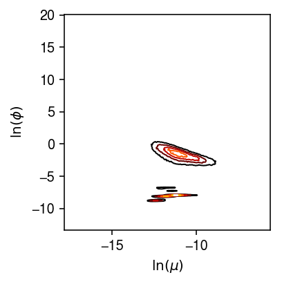
Look at zeros and dispersion.

plt.clf()
plt.gcf().set_size_inches(3, 3)
H = np.histogram2d(logodds.values.ravel(), log_phi.values.ravel(), bins=200)
X, Y = np.meshgrid(H[1], H[2])
plt.contour(X[1:,1:].T, Y[1:,1:].T, H[0], cmap=colorcet.cm['fire'], linewidths=1)
plt.xlabel('$\mathrm{logit}(\pi)$')
plt.ylabel('$\ln(\mu)$')
plt.tight_layout()

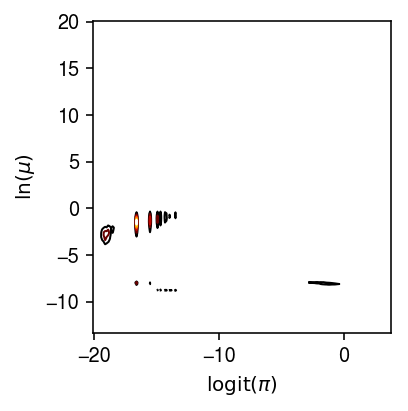
We previously looked at the relationship between estimated parameters, averaging over all 53 individuals.

Null simulation

Randomly split a homogeneous sample into two groups to generate null data sets.

def null_sim(dat, n1, n2, seed=0):
  query = sc.pp.subsample(dat, n_obs=n1 + n2, random_state=seed, copy=True)
  z = np.zeros(n1 + n2).astype(bool)
  z[:n1] = 1
  return query, z

def evaluate_null_type1(dat, n=100, min_detect=0.01, n_bootstrap=1000, n_trials=10):
  result = []
  for trial in range(n_trials):
    x, z = null_sim(dat, n, n, seed=trial)
    s = x.X.sum(axis=1).A.ravel()
    for j in range(x.shape[1]):
      diff, p = diff_var_bootstrap(x.X[:,j].A.ravel(), s, z, n_bootstrap=n_bootstrap)
      result.append(pd.Series({'trial': trial, 'gene': j, 'n': n, 'diff': diff, 'p': p}))
  result = pd.DataFrame(result)
  return result

Read 10X v3 data, which has higher sequencing depth.

dat = anndata.read_h5ad('/scratch/midway2/aksarkar/modes/10k_pbmc_v3.h5ad')

First, apply our approach to a single example.

n1 = 500
n2 = 500
x, z = null_sim(dat, n1, n2, seed=1)
s = x.X.sum(axis=1).A.ravel()
sc.pp.filter_genes(x, min_cells=0.01 * (n1 + n2))

est_diff_var(x.X[:,0].A.ravel(), s, z)

2.3068812267492158e-11

diff_var_bootstrap(x.X[:,0].A.ravel(), s, z, random_state=1)

Test the benchmark.

test_result = evaluate_null_type1(dat, n=500, n_trials=1)
test_result.head()

0 - f39f19f1-0b74-45a9-bb8b-18a9a4a3227b

Fitting kinetic models directly

Instead of assuming variance of gene expression is driven by stochastic transcription and asking whether the variance changes after some perturbation, we could attempt to ask directly whether the underlying stochastic process changes.

iPSC data

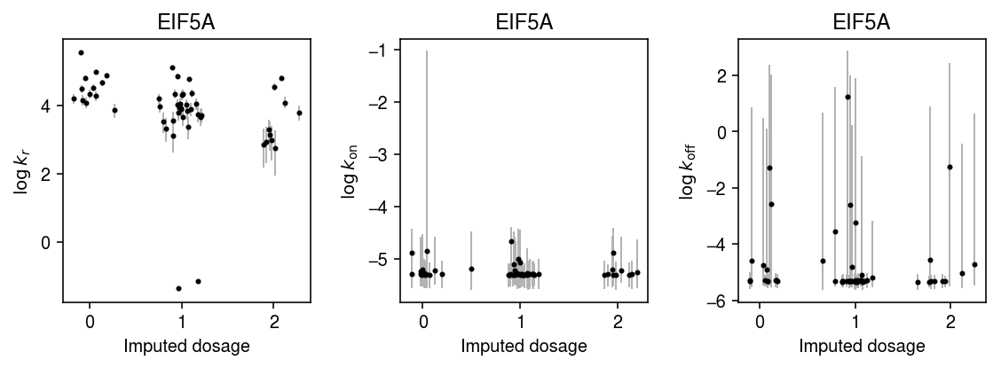
We previously identified 5 variance QTLs in iPSCs, but also found they were all mean QTLs.

Read the data.

x = anndata.read_h5ad('/project2/mstephens/aksarkar/projects/singlecell-ideas/data/ipsc/ipsc.h5ad')

vqtls = pd.read_csv('/project2/mstephens/aksarkar/projects/singlecell-qtl/data/scqtl-mapping/variance.txt.gz', sep=' ', index_col=0)

vqtls.sort_values('p_beta').head(n=5)

chr      start        end strand  num_vars  distance  \
gene
ENSG00000184674  chr22   24384681   24384680      -       477       0.0
ENSG00000113558   chr5  133512730  133512729      -       673   -2801.0
ENSG00000132507  chr17    7210319    7210318      +       496    5218.0
ENSG00000148680  chr10   92617672   92617671      -       669   47915.0
ENSG00000131469  chr17   41150291   41150290      +       515  -32887.0

id var_chr    var_start      var_end  \
gene
ENSG00000184674   esv2669470.chr22.24343050   chr22   24343050.0   24397301.0
ENSG00000113558   rs13356194.chr5.133515530    chr5  133515530.0  133515530.0
ENSG00000132507     rs1054378.chr17.7215536   chr17    7215536.0    7215536.0
ENSG00000148680  rs138704692.chr10.92569757   chr10   92569757.0   92569757.0
ENSG00000131469   rs12947287.chr17.41117404   chr17   41117404.0   41117404.0

df    dummy         a        b     p_nominal      beta  \
gene
ENSG00000184674  51.0  43.2504  1.033960  59.1680  4.192900e-11 -1.182590
ENSG00000113558  51.0  39.5051  1.066360  37.1031  1.387570e-10 -0.796700
ENSG00000132507  51.0  42.2941  1.069530  73.9335  7.525920e-10 -1.214550
ENSG00000148680  51.0  42.9914  1.035830  43.6306  4.632030e-09 -1.044440
ENSG00000131469  51.0  34.8434  0.902717  23.8075  8.796860e-11 -0.848284

p_empirical        p_beta
gene
ENSG00000184674       0.0001  4.266760e-08
ENSG00000113558       0.0001  2.371110e-07
ENSG00000132507       0.0001  6.094700e-07
ENSG00000148680       0.0001  2.088450e-06
ENSG00000131469       0.0001  7.746900e-06

x.var.loc['ENSG00000184674']

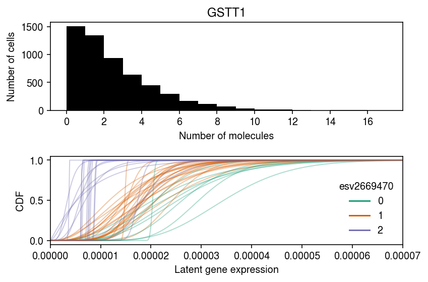
chr             hs22
start       24376133
end         24384680
name           GSTT1
strand             -
source    H. sapiens
Name: ENSG00000184674, dtype: object

with sqlite3.connect('/project2/mstephens/aksarkar/projects/singlecell-qtl/browser/browser.db') as conn:
  geno = pd.read_sql('select * from mean_qtl_geno where gene = ?', con=conn, params=('ENSG00000184674',)).set_index('ind')['value']

Read the previously fitted point-Gamma distribution for each individual.

log_mu = pd.read_csv('/project2/mstephens/aksarkar/projects/singlecell-qtl/data/density-estimation/design1/zi2-log-mu.txt.gz', sep=' ', index_col=0)
log_phi = pd.read_csv('/project2/mstephens/aksarkar/projects/singlecell-qtl/data/density-estimation/design1/zi2-log-phi.txt.gz', sep=' ', index_col=0)
logodds = pd.read_csv('/project2/mstephens/aksarkar/projects/singlecell-qtl/data/density-estimation/design1/zi2-logodds.txt.gz', sep=' ', index_col=0)

Plot the observed data and the fitted distributions.

query = x.X.tocsc()[:,(x.var['name'] == 'GSTT1').values].A.ravel()
lam = query / x.obs['mol_hs']

cm = plt.get_cmap('Dark2')
k = 'ENSG00000184674'

plt.clf()
fig, ax = plt.subplots(2, 1)
fig.set_size_inches(6, 4)
bins = np.arange(query.max() + 1)
ax[0].hist(query, bins=bins, color='k')
ax[0].set_xlabel('Number of molecules')
ax[0].set_ylabel('Number of cells')
ax[0].set_title(x.var.loc[k, 'name'])
ax[0].set_xticks(bins[::2])

grid = np.linspace(0, lam.max(), 1000)
for i in log_mu.columns:
  if i in geno.index:
    t = log_mu.loc[k, i], log_phi.loc[k, i], logodds.loc[k, i]
    F = st.gamma(a=np.exp(-t[1]), scale=np.exp(t[0] + t[1])).cdf(grid)
    # Important: we need to round the imputed dosages
    ax[1].plot(grid, F, lw=1, alpha=0.35, c=cm(int(np.round(geno.loc[i]))))
dummy = [plt.Line2D([0], [0], c=cm(i)) for i in range(3)]
ax[1].legend(dummy, np.arange(3), title=vqtls.loc[k, 'id'].split('.')[0], frameon=False)
ax[1].set_xlabel('Latent gene expression')
ax[1].set_ylabel('CDF')
ax[1].set_xlim(0, 7e-5)

fig.tight_layout()

Estimate the posterior distribution of kinetic parameters for each individual.

k_params = dict()
for i in geno.index:
  print(f'Fitting individual {i}')
  keep = (x.obs['chip_id'] == i).values.ravel()
  xg = query[keep]
  sg = x.obs['mol_hs'].values[keep]
  samples, _ = poisbeta.fit_poisson_beta_mcmc(xg, n_samples=1000, ar=1, br=xg.max(), aon=1, bon=100, aoff=1, boff=100)
  k_params[i] = samples

Write out the samples.

with open('/scratch/midway2/aksarkar/ideas/ipsc-gstt1-post.pkl', 'wb') as f:
  pickle.dump(k_params, f)

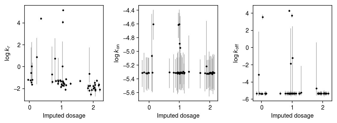
Plot the 95% credible intervals for each parameter in each individual, against genotype.

plt.clf()
fig, ax = plt.subplots(1, 3)
fig.set_size_inches(8, 3)
n = geno.shape[0]
for j, (a, t) in enumerate(zip(ax, ['$\log\,k_r$', '$\log\,k_{\mathrm{on}}$', '$\log\,k_{\mathrm{off}}$'])):
  y = np.array([np.log(k_params[i][-800:,j]).mean() for i in geno.index])
  ci = np.array([np.percentile(np.log(k_params[i][-800:,j]), [2.5, 97.5]) for i in geno.index]).T
  ax[j].errorbar(x=geno.values + np.random.normal(scale=0.1, size=n),
                 y=y,
                 yerr=abs(ci - y),
                 fmt='.',
                 c='k',
                 ecolor='0.7',
                 elinewidth=1,
                 ms=4,
  )
  ax[j].set_xlabel('Imputed dosage')
  ax[j].set_ylabel(t)
  fig.tight_layout()

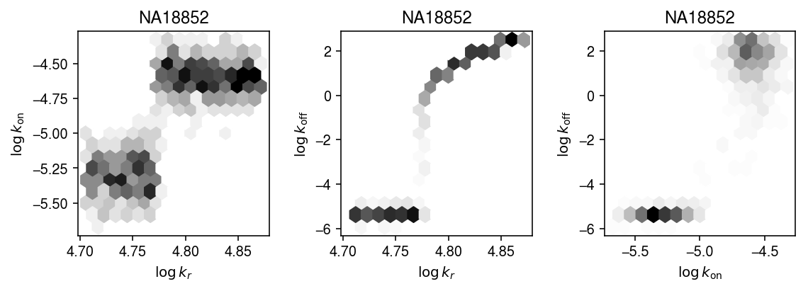
Plot one of the joint posteriors.

names = ['$\log\,k_r$', '$\log\,k_{\mathrm{on}}$', '$\log\,k_{\mathrm{off}}$']
plt.clf()
fig, ax = plt.subplots(1, 3)
fig.set_size_inches(8, 3)
for (s, t), a in zip(it.combinations(range(3), 2), ax):
  x = np.array([np.log(k_params['NA18852'][-800:,s]) for i in geno.index])
  y = np.array([np.log(k_params['NA18852'][-800:,t]) for i in geno.index])
  a.hexbin(x=x, y=y, gridsize=15, cmap=colorcet.cm['gray_r'])
  a.set_xlabel(names[s])
  a.set_ylabel(names[t])
  a.set_title('NA18852')
fig.tight_layout()

Repeat the analysis for the rest of the vQTLs.

k = 'ENSG00000113558'
with sqlite3.connect('/project2/mstephens/aksarkar/projects/singlecell-qtl/browser/browser.db') as conn:
  geno = pd.read_sql('select * from mean_qtl_geno where gene = ?', con=conn, params=(k,)).set_index('ind')['value']
query = x.X.tocsc()[:,list(x.var.index).index(k)].A.ravel()
k_params = dict()
for i in geno.index:
  print(f'Fitting individual {i}')
  keep = (x.obs['chip_id'] == i).values.ravel()
  xg = query[keep]
  sg = x.obs['mol_hs'].values[keep]
  samples, _ = poisbeta.fit_poisson_beta_mcmc(xg, n_samples=1000, ar=1, br=xg.max(), aon=1, bon=100, aoff=1, boff=100)
  k_params[i] = samples

plt.clf()
fig, ax = plt.subplots(1, 3)
fig.set_size_inches(8, 3)
n = geno.shape[0]
for j, (a, t) in enumerate(zip(ax, ['$\log\,k_r$', '$\log\,k_{\mathrm{on}}$', '$\log\,k_{\mathrm{off}}$'])):
  y = np.array([np.log(k_params[i][-800:,j]).mean() for i in geno.index])
  ci = np.array([np.percentile(np.log(k_params[i][-800:,j]), [2.5, 97.5]) for i in geno.index]).T
  ax[j].errorbar(x=geno.values + np.random.normal(scale=0.1, size=n),
                 y=y,
                 yerr=abs(ci - y),
                 fmt='.',
                 c='k',
                 ecolor='0.7',
                 elinewidth=1,
                 ms=4,
  )
  ax[j].set_title(x.var.loc['ENSG00000113558', 'name'])
  ax[j].set_xlabel('Imputed dosage')
  ax[j].set_ylabel(t)
  fig.tight_layout()

k = 'ENSG00000132507'
with sqlite3.connect('/project2/mstephens/aksarkar/projects/singlecell-qtl/browser/browser.db') as conn:
  geno = pd.read_sql('select * from mean_qtl_geno where gene = ?', con=conn, params=(k,)).set_index('ind')['value']
query = x.X.tocsc()[:,list(x.var.index).index(k)].A.ravel()
k_params = dict()
for i in geno.index:
  print(f'Fitting individual {i}')
  keep = (x.obs['chip_id'] == i).values.ravel()
  xg = query[keep]
  sg = x.obs['mol_hs'].values[keep]
  samples, _ = poisbeta.fit_poisson_beta_mcmc(xg, n_samples=1000, ar=1, br=xg.max(), aon=1, bon=100, aoff=1, boff=100)
  k_params[i] = samples

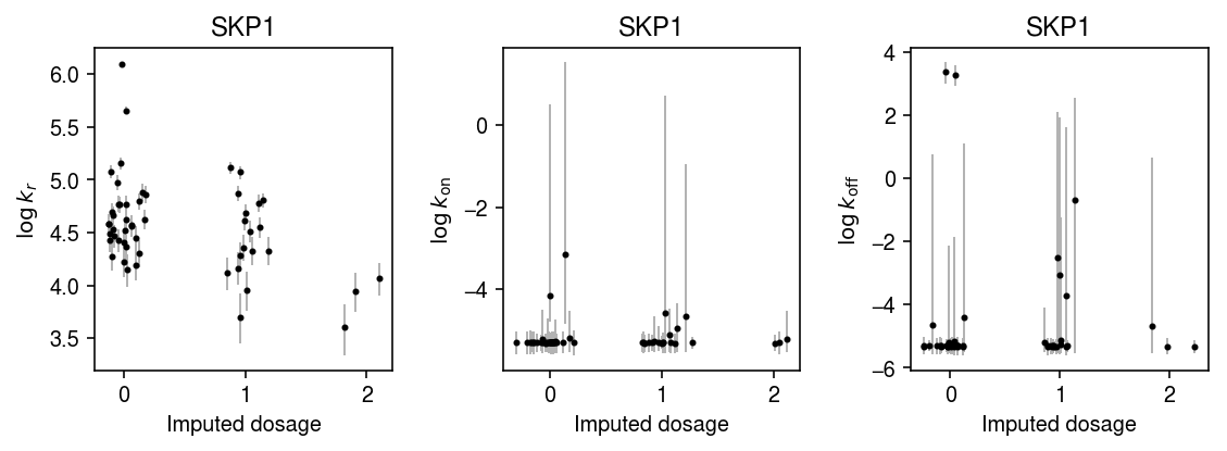
plt.clf()
fig, ax = plt.subplots(1, 3)
fig.set_size_inches(8, 3)
n = geno.shape[0]
for j, (a, t) in enumerate(zip(ax, ['$\log\,k_r$', '$\log\,k_{\mathrm{on}}$', '$\log\,k_{\mathrm{off}}$'])):
  y = np.array([np.log(k_params[i][-800:,j]).mean() for i in geno.index])
  ci = np.array([np.percentile(np.log(k_params[i][-800:,j]), [2.5, 97.5]) for i in geno.index]).T
  ax[j].errorbar(x=geno.values + np.random.normal(scale=0.1, size=n),
                 y=y,
                 yerr=abs(ci - y),
                 fmt='.',
                 c='k',
                 ecolor='0.7',
                 elinewidth=1,
                 ms=4,
  )
  ax[j].set_title(x.var.loc[k, 'name'])
  ax[j].set_xlabel('Imputed dosage')
  ax[j].set_ylabel(t)
  fig.tight_layout()

iPSC-CM time course data

Selewa et al. 2019 generated Drop-Seq of iPSCs differentiating into cardiomyocytes at days 0, 1, 3, 7, and 15. Read the data.

counts = si.mmread('/project2/mstephens/aksarkar/projects/singlecell-ideas/data/czi/drop/counts.mtx.gz')
genes = pd.read_table('/project2/mstephens/aksarkar/projects/singlecell-ideas/data/czi/drop/genes.txt', header=None)
genes.columns = ['name']
cells = pd.read_table('/project2/mstephens/aksarkar/projects/singlecell-ideas/data/czi/drop/cells.txt', sep=' ')
cells.columns = ['barcode', 'day', 'ind']
cells['day'] = pd.Categorical(cells['day'])
x = anndata.AnnData(counts.T.tocsc(), obs=cells, var=genes)
x.write('/project2/mstephens/aksarkar/projects/singlecell-ideas/data/czi/drop/czi-ipsc-cm.h5ad')

y = x[x.obs['ind'] == 'Rep1']
sc.pp.filter_genes(y, min_counts=.01 * y.shape[0])
y.var = y.var.reset_index(drop=True)
y.shape
y.write('/project2/mstephens/aksarkar/projects/singlecell-ideas/data/czi/drop/czi-ipsc-cm-rep1.h5ad')

y = anndata.read_h5ad('/project2/mstephens/aksarkar/projects/singlecell-ideas/data/czi/drop/czi-ipsc-cm-rep1.h5ad')

Fit a fully unsupervised NMF model to achieve two goals:

Merge cells across time points which are in the same cell state
Cluster cells within/across time points to separate cell states

m = skd.NMF(n_components=10, beta_loss=1, solver='mu', init='random', max_iter=1000)
l = m.fit_transform(y.X)
f = m.components_

Normalize the NMF solution into a topic model.

weights = l * f.sum(axis=1)
scale = weights.sum(axis=1, keepdims=True)
weights /= scale
topics = f / f.sum(axis=1, keepdims=True)

Write out the topic model.

np.save('/scratch/midway2/aksarkar/ideas/ipsc-cm-topic-weights.npz', weights)
np.save('/scratch/midway2/aksarkar/ideas/ipsc-cm-topics.npz', topics)
np.save('/scratch/midway2/aksarkar/ideas/ipsc-cm-topic-scale.npz', scale)

First, compute the correlation matrix between the topic weights and the day of the protocol.

r = np.corrcoef(pd.get_dummies(y.obs['day']).T, weights.T)[:10,:4]
plt.clf()
plt.gcf().set_size_inches(4, 4)
plt.imshow(r, cmap=colorcet.cm['coolwarm'], vmin=-1, vmax=1)
plt.xlabel('Day')
plt.xticks(np.arange(4), y.obs['day'].cat.categories)
plt.ylabel('Topic')
plt.yticks(np.arange(10), 1 + np.arange(10))
cb = plt.colorbar()
cb.set_label('Correlation')
plt.tight_layout()

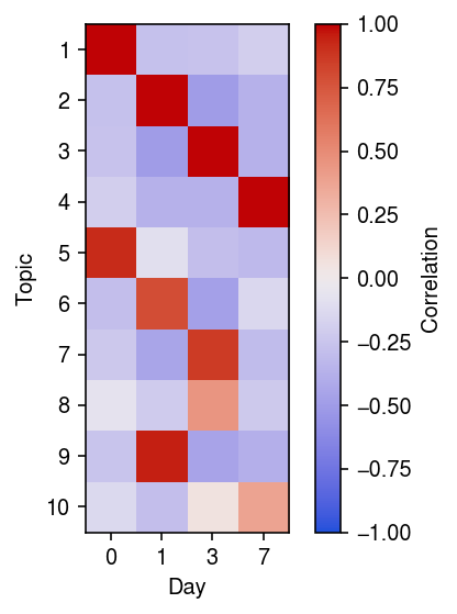
We might expect (from a pseudotime perspective) that there are cells “between” days, which would have non-trivial topic weight in multiple days. If there were such cells, we might expect weak positive correlations between multiple days and topics; however, we find only one such topic.

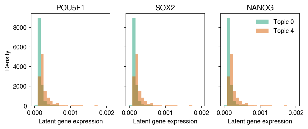
Interestingly, we also find multiple topics correlated with each day. To begin with, examine topics 0 and 4 (which correlate with day 0), and look at expression of pluritpotency markers in cells with maximal topic weight in those topics.

lam = l @ f
lam /= y.X.sum(axis=1)

cm = plt.get_cmap('Dark2')
plt.clf()
fig, ax = plt.subplots(1, 3, sharey=True)
fig.set_size_inches(7, 3)
for a, k in zip(ax, ['POU5F1', 'SOX2', 'NANOG']):
  idx = y.var[y.var['name'] == k].reset_index(drop=True).index.astype(int)
  for j, topic in enumerate([0, 4]):
    query = lam[np.where(np.argmax(weights, 1) == j)[0],idx]
    a.hist(query, density=True, bins=np.linspace(0, 2e-3, 25), alpha=0.5, color=cm(j), label=f'Topic {topic}')
  a.set_xlabel('Latent gene expression')
  a.set_title(k)
ax[0].set_ylabel('Density')
ax[-1].legend(frameon=False)
fig.tight_layout()

Based on the topic model, we might safely begin by just analyzing each time point as a homogeneous collection of cells. Estimate gene expression mean and variance for each gene in each time point.

point_gamma_res = dict()
for k in (0, 1, 3, 7):
  point_gamma_res[k] = scmodes.ebpm.sgd.ebpm_point_gamma(
    y.X[y.obs['day'] == k],
    lr=1e-2, batch_size=128, max_epochs=20, verbose=True)

res = pd.concat({k: pd.DataFrame(np.vstack(v[:-1]).T,
                                 columns=['log_mu', 'neg_log_phi', 'logodds'])
                  for k, v in point_gamma_res.items()}, axis='columns')
res.to_csv('/scratch/midway2/aksarkar/ideas/ipsc-cm-ebpm-point-gamma.txt.gz')

res = pd.read_csv('/scratch/midway2/aksarkar/ideas/ipsc-cm-ebpm-point-gamma.txt.gz', index_col=0, header=[0, 1])

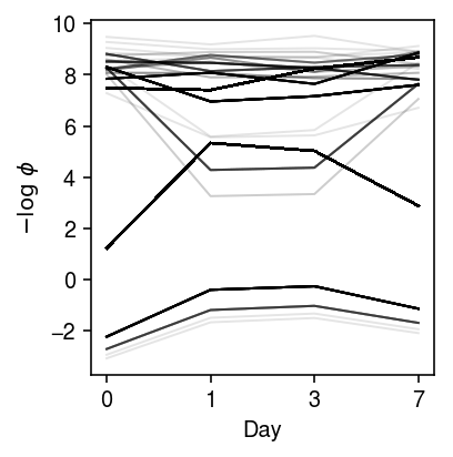
Look at the trajectories of dispersion over time.

plt.clf()
plt.gcf().set_size_inches(3, 3)
for k, z in res.loc(axis=1)[:,'neg_log_phi'].iterrows():
  if z.mean() > -10:
    plt.plot(z.values.ravel(), c='k', lw=1, alpha=0.1)
plt.xlabel('Day')
plt.xticks(np.arange(4), [0, 1, 3, 7])
plt.ylabel('$-\log\ \phi$')
plt.tight_layout()

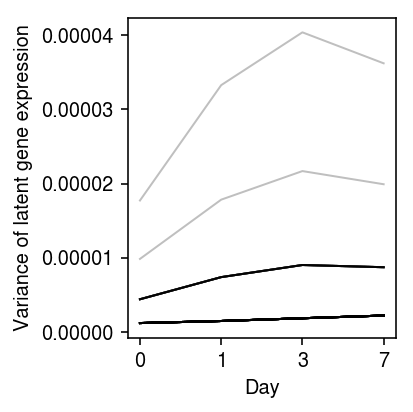
Look at the trajectories of variance over time.

plt.clf()
plt.gcf().set_size_inches(3, 3)
for k, z in res.iterrows():
  var = np.exp(2 * z.loc[:,'log_mu'] - z.loc[:,'neg_log_phi'])
  if np.median(var) > 1e-6:
    plt.plot(var.values.ravel(), c='k', lw=1, alpha=0.25)
plt.xlabel('Day')
plt.xticks(np.arange(4), [0, 1, 3, 7])
plt.ylabel('Variance of latent gene expression')
plt.tight_layout()

Extract some interesting examples.

res[np.logical_and(res.loc(axis=1)['0', 'neg_log_phi'] < 2, res.loc(axis=1)['1', 'neg_log_phi'] > 2)].head()

0                               1                               3  \
log_mu neg_log_phi   logodds    log_mu neg_log_phi   logodds    log_mu
38  -8.624235    1.224293 -8.834169 -7.599703    5.335293 -9.648245 -7.419324
127 -8.624235    1.224293 -8.834169 -7.599703    5.335293 -9.648245 -7.419324
254 -8.624235    1.224293 -8.834169 -7.599703    5.335293 -9.648245 -7.419324
286 -8.624235    1.224293 -8.834169 -7.599703    5.335293 -9.648245 -7.419324
320 -8.624235    1.224293 -8.834169 -7.599703    5.335293 -9.648245 -7.419324

7
neg_log_phi   logodds    log_mu neg_log_phi   logodds
38     5.027008 -9.271143 -7.770187      2.8829 -8.345497
127    5.027008 -9.271143 -7.770187      2.8829 -8.345497
254    5.027008 -9.271143 -7.770187      2.8829 -8.345497
286    5.027008 -9.271143 -7.770187      2.8829 -8.345497
320    5.027008 -9.271143 -7.770187      2.8829 -8.345497

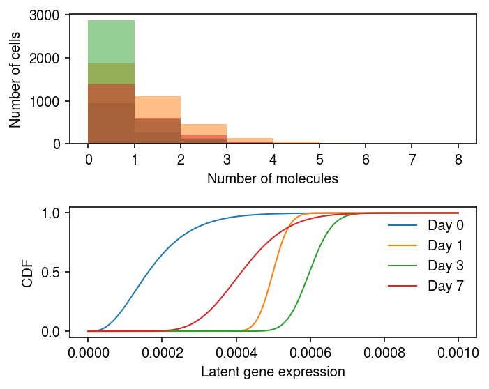
NDUFAB1 appears to show a reduction in variance between days 0 and 1, and then a subsequent gain in variance between days 3 and 7.

y.var.iloc[38]

name        NDUFAB1
n_counts       5571
Name: 49, dtype: object

Plot the data and the fitted distributions

plt.set_cmap('Dark2')
plt.clf()
fig, ax = plt.subplots(2, 1)
fig.set_size_inches(5, 4)

days = [0, 1, 3, 7]
query = y.X[:,38].A.ravel()
bins = np.arange(query.max() + 1)
for i, k in enumerate(days):
  ax[0].hist(query[y.obs['day'] == k], bins=bins, color=f'C{i}', alpha=0.5)
ax[0].set_xlabel('Number of molecules')
ax[0].set_ylabel('Number of cells')

grid = np.linspace(0, 1e-3, 1000)
for i, k in enumerate([str(d) for d in days]):
  log_mu = res.loc[38, (k, 'log_mu')]
  neg_log_phi = res.loc[38, (k, 'neg_log_phi')]
  logodds = res.loc[38, (k, 'logodds')]
  F = st.gamma(a=np.exp(neg_log_phi), scale=np.exp(log_mu - neg_log_phi)).cdf(grid)
  F = sp.expit(logodds) + sp.expit(-logodds) * F
  ax[1].plot(grid, F, lw=1, color=f'C{i}', label=f'Day {k}')
ax[1].legend(frameon=False)
ax[1].set_xlabel('Latent gene expression')
ax[1].set_ylabel('CDF')
fig.tight_layout()

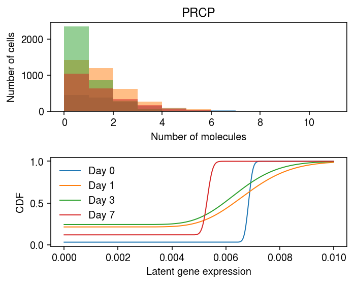
Look at examples with the opposite trajectory.

res[np.logical_and(res.loc(axis=1)['0', 'neg_log_phi'] > 8, res.loc(axis=1)['1', 'neg_log_phi'] < 4)].head()

0                              1                               3  \
log_mu neg_log_phi   logodds   log_mu neg_log_phi   logodds    log_mu
5851 -4.983784    8.014603 -3.454462 -4.98496    3.259651 -1.306795 -5.037562
6641 -4.983784    8.014603 -3.454462 -4.98496    3.259651 -1.306795 -5.037562

7
neg_log_phi   logodds    log_mu neg_log_phi   logodds
5851    3.340554 -1.143311 -5.236426    7.055284 -2.009873
6641    3.340554 -1.143311 -5.236426    7.055284 -2.009873

x.var.iloc[[5851, 6641]]

name
5851   PRCP
6641  UBXN4

plt.set_cmap('Dark2')
plt.clf()
fig, ax = plt.subplots(2, 1)
fig.set_size_inches(5, 4)

days = [0, 1, 3, 7]
query = y.X[:,(y.var['name'] == 'PRCP').values].A.ravel()
bins = np.arange(query.max() + 1)
for i, k in enumerate(days):
  ax[0].hist(query[y.obs['day'] == k], bins=bins, color=f'C{i}', alpha=0.5)
ax[0].set_xlabel('Number of molecules')
ax[0].set_ylabel('Number of cells')
ax[0].set_title(x.var.iloc[idx][0])

grid = np.linspace(0, 1e-2, 1000)
for i, k in enumerate([str(d) for d in days]):
  log_mu = res.loc[idx, (k, 'log_mu')]
  neg_log_phi = res.loc[idx, (k, 'neg_log_phi')]
  logodds = res.loc[idx, (k, 'logodds')]
  F = st.gamma(a=np.exp(neg_log_phi), scale=np.exp(log_mu - neg_log_phi)).cdf(grid)
  F = sp.expit(logodds) + sp.expit(-logodds) * F
  ax[1].plot(grid, F, lw=1, color=f'C{i}', label=f'Day {k}')
ax[1].legend(frameon=False)
ax[1].set_xlabel('Latent gene expression')
ax[1].set_ylabel('CDF')
fig.tight_layout()

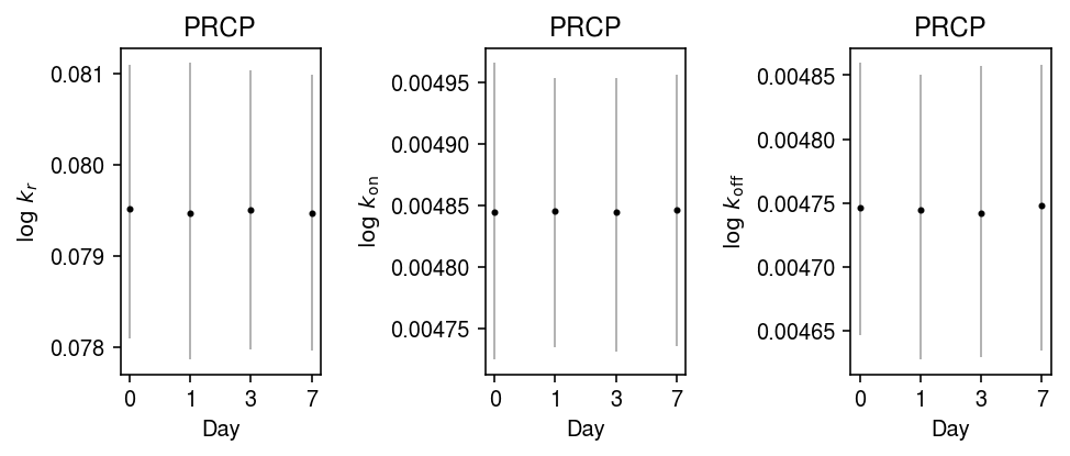
Fit kinetic models for PRCP gene expression at each time point.

idx = 5851
k_params = dict()
traces = dict()
for k in [0, 1, 3, 7]:
  print(f'Fitting day {k}')
  query = y.X[:,idx].A.ravel()
  # Default hyperparameters follow Kim & Marioni 2013
  samples, trace = poisbeta.fit_poisson_beta_mcmc(query, n_samples=1000)
  k_params[k] = samples
  traces[k] = trace

with open('/scratch/midway2/aksarkar/ideas/ipsc-cm-mcmc.pkl', 'wb') as f:
  pickle.dump((k_params, traces), f)

with open('/scratch/midway2/aksarkar/ideas/ipsc-cm-mcmc.pkl', 'rb') as f:
  k_params, traces = pickle.load(f)

mcmc_res = pd.concat({k: pd.DataFrame(k_params[k], columns=['log_k_r', 'log_k_on', 'log_k_koff']) for k in k_params}, axis='columns')

plt.clf()
fig, ax = plt.subplots(1, 3)
fig.set_size_inches(7, 3)
for a, k, t in zip(ax, ['log_k_r', 'log_k_on', 'log_k_koff'], ['$\log\ k_r$', '$\log\ k_{\mathrm{on}}$', '$\log\ k_{\mathrm{off}}$']):
  samples = mcmc_res.loc(axis=1)[:,k][-800:]
  pm = samples.mean()
  a.errorbar(x=np.arange(4),
             y=pm,
             yerr=abs(np.percentile(samples, [2.5, 97.5], axis=0) - pm.values.reshape(1, -1)),
             fmt='.',
             c='k',
             ecolor='0.7',
             elinewidth=1,
             ms=4,)
  a.set_xlabel('Day')
  a.set_xticks(np.arange(4))
  a.set_xticklabels([0, 1, 3, 7])
  a.set_ylabel(t)
  a.set_title(y.var.loc[str(idx), 'name'])
fig.tight_layout()

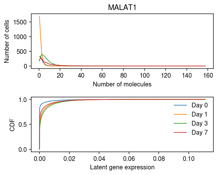
Look at the most variable gene.

order = np.argsort(-np.median(np.exp(2 * res.loc(axis=1)[:,'log_mu'].values - res.loc(axis=1)[:,'neg_log_phi'].values), axis=1))[:10]
y.var.loc[order]

name  n_counts
10227   MALAT1   53633.0
3178    EXOSC8    5236.0
8226    RPL35A   36692.0
8929    RPL37A   29614.0
9331   MT-ND4L   12695.0
8645    COMMD6    6545.0
2993     RPS25   11410.0
10449   MRPS21    9434.0
7942     DDX10    1003.0
2640   SELENOK    2380.0

plt.set_cmap('Dark2')
plt.clf()
fig, ax = plt.subplots(2, 1)
fig.set_size_inches(5, 4)

idx = 10227
days = [0, 1, 3, 7]
query = y.X[:,idx].A.ravel()
bins = np.arange(query.max() + 1)
for i, k in enumerate(days):
  h, e = np.histogram(query[y.obs['day'] == k], bins=bins)
  ax[0].plot(bins[:-1] + 0.5, h, color=f'C{i}', lw=1)
ax[0].set_xlabel('Number of molecules')
ax[0].set_ylabel('Number of cells')
ax[0].set_title(y.var.iloc[idx]['name'])

lam = query / y.X.sum(axis=1).A.ravel()
grid = np.linspace(lam.min(), lam.max(), 1000)
for i, k in enumerate([str(d) for d in days]):
  log_mu = res.loc[idx, (k, 'log_mu')]
  neg_log_phi = res.loc[idx, (k, 'neg_log_phi')]
  logodds = res.loc[idx, (k, 'logodds')]
  F = st.gamma(a=np.exp(neg_log_phi), scale=np.exp(log_mu - neg_log_phi)).cdf(grid)
  F = sp.expit(logodds) + sp.expit(-logodds) * F
  ax[1].plot(grid, F, lw=1, color=f'C{i}', label=f'Day {k}')
ax[1].legend(frameon=False)
ax[1].set_xlabel('Latent gene expression')
ax[1].set_ylabel('CDF')
fig.tight_layout()

Variational inference

Null simulation

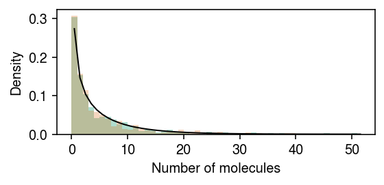
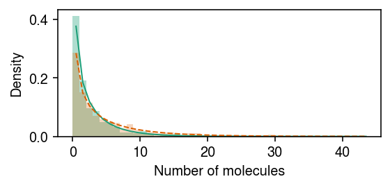
Simulate from the model, fixing \(\delmu = \delphi = 0\).

rng = np.random.default_rng(1)
n = 500
log_mean = -10
log_inv_disp = -0.5
lam = rng.gamma(shape=np.exp(log_inv_disp), scale=np.exp(log_mean - log_inv_disp), size=2 * n)
s = np.full(2 * n, 1e5)
x = rng.poisson(s * lam)
z = np.zeros(2 * n, dtype=bool)
z[:n] = 1

Plot the simulated data.

cm = plt.get_cmap('Dark2')
plt.clf()
plt.gcf().set_size_inches(4, 2)
grid = np.arange(x.max() + 2)
plt.hist(x[z], bins=grid, color=cm(0), density=True, alpha=0.35)
plt.hist(x[~z], bins=grid, color=cm(1), density=True, alpha=0.25)
plt.plot(grid + .5, st.nbinom(n=np.exp(log_inv_disp), p=1 / (1 + s[0] * np.exp(log_mean - log_inv_disp))).pmf(grid), c='k', lw=1)
plt.xlabel('Number of molecules')
plt.ylabel('Density')
plt.tight_layout()

Fit the model.

n_epochs = 2000
n_samples = 10
run = 0
fit0 = scmodes.ebpm.ebpm_gamma(x, s)
torch.manual_seed(run)
m = DiffVarExprModel(
  prior_log_mean=torch.distributions.Normal(loc=fit0[0], scale=1.),
  prior_log_inv_disp=torch.distributions.Normal(loc=fit0[1], scale=1.))
m.fit(
  torch.tensor(x.reshape(-1, 1), dtype=torch.float),
  torch.tensor(s.reshape(-1, 1), dtype=torch.float),
  torch.tensor(z.reshape(-1, 1), dtype=torch.float),
  n_epochs=n_epochs,
  n_samples=n_samples,
  log_dir=f'/scratch/midway2/aksarkar/singlecell/runs/diffvar/dev_nb_{n_epochs}_{n_samples}_{run}')

DiffVarExprModel()

Plot the fit.

cm = plt.get_cmap('Dark2')
plt.clf()
plt.gcf().set_size_inches(4, 2)
grid = np.arange(x.max() + 2)
plt.hist(x[z], bins=grid, color=cm(0), density=True, alpha=0.35)
plt.plot(grid + .5, st.nbinom(n=np.exp(m.log_inv_disp[0]), p=1 / (1 + s[0] * np.exp(m.log_mean[0] - m.log_inv_disp[0]))).pmf(grid), c=cm(0), lw=1)
plt.hist(x[~z], bins=grid, color=cm(1), density=True, alpha=0.25)
plt.plot(grid + .5, st.nbinom(n=np.exp(m.log_inv_disp[0] - m.diff_inv_disp[0]), p=1 / (1 + s[0] * np.exp(m.log_mean[0] - m.log_inv_disp[0] - m.diff_mean[0] - m.diff_inv_disp[0]))).pmf(grid), c=cm(1), lw=1, ls='--')
plt.xlabel('Number of molecules')
plt.ylabel('Density')
plt.tight_layout()

Report the LFSR for DE/DD.

pd.Series({
  'de': m.lfsr_diff_mean[0],
  'dd': m.lfsr_diff_inv_disp[0]
})

de    0.426195
dd    0.305537
dtype: float64

DE

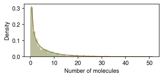
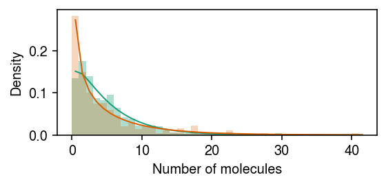
Simulate data under differential expression, but not differential dispersion.

rng = np.random.default_rng(1)
n = 500
z = np.zeros(2 * n, dtype=bool)
z[:n] = 1
log_mean = -10
log_inv_disp = -0.5
diff_mean = np.log(2)
lam = rng.gamma(shape=np.exp(log_inv_disp), scale=np.exp(log_mean - log_inv_disp - z * diff_mean), size=2 * n)
s = np.full(2 * n, 1e5)
x = rng.poisson(s * lam)

Plot the simulated data.

cm = plt.get_cmap('Dark2')
plt.clf()
plt.gcf().set_size_inches(4, 2)
grid = np.arange(x.max() + 2)
plt.hist(x[z], bins=grid, color=cm(0), density=True, alpha=0.35)
plt.plot(grid + .5, st.nbinom(n=np.exp(log_inv_disp), p=1 / (1 + s[0] * np.exp(log_mean - log_inv_disp - diff_mean))).pmf(grid), c=cm(0), lw=1)
plt.hist(x[~z], bins=grid, color=cm(1), density=True, alpha=0.25)
plt.plot(grid + .5, st.nbinom(n=np.exp(log_inv_disp), p=1 / (1 + s[0] * np.exp(log_mean - log_inv_disp))).pmf(grid), c=cm(1), lw=1)
plt.xlabel('Number of molecules')
plt.ylabel('Density')
plt.tight_layout()

Fit the model.

n_epochs = 2000
n_samples = 10
run = 0
fit0 = scmodes.ebpm.ebpm_gamma(x, s)
torch.manual_seed(run)
m = DiffVarExprModel(
  prior_log_mean=torch.distributions.Normal(loc=fit0[0], scale=1.),
  prior_log_inv_disp=torch.distributions.Normal(loc=fit0[1], scale=1.))
m.fit(
  torch.tensor(x.reshape(-1, 1), dtype=torch.float),
  torch.tensor(s.reshape(-1, 1), dtype=torch.float),
  torch.tensor(z.reshape(-1, 1), dtype=torch.float),
  n_epochs=n_epochs,
  n_samples=n_samples,
  log_dir=f'/scratch/midway2/aksarkar/singlecell/runs/diffvar/dev_nb_2fold_{n_epochs}_{n_samples}_{run}')

DiffVarExprModel()

Plot the fit.

cm = plt.get_cmap('Dark2')
plt.clf()
plt.gcf().set_size_inches(4, 2)
grid = np.arange(x.max() + 2)
plt.hist(x[z], bins=grid, color=cm(0), density=True, alpha=0.35)
plt.plot(grid + .5, st.nbinom(
  n=np.exp(m.log_inv_disp[0] + m.diff_inv_disp[0]),
  p=1 / (1 + s[0] * np.exp(m.log_mean[0] - m.log_inv_disp[0] + m.diff_mean[0] + m.diff_inv_disp[0]))).pmf(grid), c=cm(0), lw=1)
plt.hist(x[~z], bins=grid, color=cm(1), density=True, alpha=0.25)
plt.plot(grid + .5, st.nbinom(
  n=np.exp(m.log_inv_disp[0]),
  p=1 / (1 + s[0] * np.exp(m.log_mean[0] - m.log_inv_disp[0]))).pmf(grid), c=cm(1), lw=1, ls='--')
plt.xlabel('Number of molecules')
plt.ylabel('Density')
plt.tight_layout()

Report the lfsr for DE/DD.

pd.Series({
  'de': m.lfsr_diff_mean[0],
  'dd': m.lfsr_diff_inv_disp[0]
})

de    3.836553e-25
dd    3.287435e-01
dtype: float64

DD

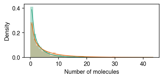
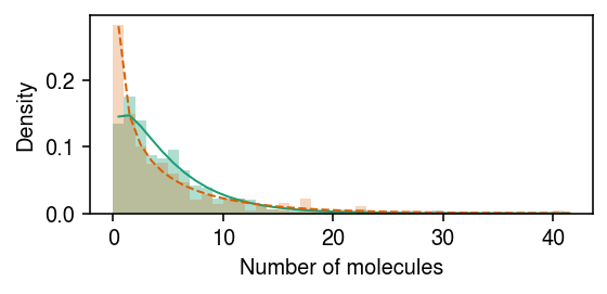
Simulate data under differential dispersion, but not differential expression.

rng = np.random.default_rng(1)
n = 500
z = np.zeros(2 * n, dtype=bool)
z[:n] = 1
log_mean = -10
log_inv_disp = -0.5
diff_inv_disp = np.log(2)
lam = rng.gamma(shape=np.exp(log_inv_disp + z * diff_inv_disp), scale=np.exp(log_mean - log_inv_disp - z * diff_inv_disp), size=2 * n)
s = np.full(2 * n, 1e5)
x = rng.poisson(s * lam)

Plot the simulated data.

cm = plt.get_cmap('Dark2')
plt.clf()
plt.gcf().set_size_inches(4, 2)
grid = np.arange(x.max() + 2)
plt.hist(x[z], bins=grid, color=cm(0), density=True, alpha=0.35)
plt.plot(grid + .5, st.nbinom(n=np.exp(log_inv_disp + diff_inv_disp), p=1 / (1 + s[0] * np.exp(log_mean - log_inv_disp - diff_inv_disp))).pmf(grid), c=cm(0), lw=1)
plt.hist(x[~z], bins=grid, color=cm(1), density=True, alpha=0.25)
plt.plot(grid + .5, st.nbinom(n=np.exp(log_inv_disp), p=1 / (1 + s[0] * np.exp(log_mean - log_inv_disp))).pmf(grid), c=cm(1), lw=1)
plt.xlabel('Number of molecules')
plt.ylabel('Density')
plt.tight_layout()

Fit the model.

n_epochs = 2000
n_samples = 10
run = 0
fit0 = scmodes.ebpm.ebpm_gamma(x, s)
torch.manual_seed(run)
m = DiffVarExprModel(
  prior_log_mean=torch.distributions.Normal(loc=fit0[0], scale=1.),
  prior_log_inv_disp=torch.distributions.Normal(loc=fit0[1], scale=1.))
m.fit(
  torch.tensor(x.reshape(-1, 1), dtype=torch.float),
  torch.tensor(s.reshape(-1, 1), dtype=torch.float),
  torch.tensor(z.reshape(-1, 1), dtype=torch.float),
  n_epochs=n_epochs,
  n_samples=n_samples,
  log_dir=f'/scratch/midway2/aksarkar/singlecell/runs/diffvar/dev_nb_dd_2fold_{n_epochs}_{n_samples}_{run}')

DiffVarExprModel()

Plot the fit.

cm = plt.get_cmap('Dark2')
plt.clf()
plt.gcf().set_size_inches(4, 2)
grid = np.arange(x.max() + 2)
plt.hist(x[z], bins=grid, color=cm(0), density=True, alpha=0.35)
plt.plot(grid + .5, st.nbinom(
  n=np.exp(m.log_inv_disp[0] - m.diff_inv_disp[0]),
  p=1 / (1 + s[0] * np.exp(m.log_mean[0] - m.log_inv_disp[0] + m.diff_mean[0] + m.diff_inv_disp[0]))).pmf(grid), c=cm(0), lw=1)
plt.hist(x[~z], bins=grid, color=cm(1), density=True, alpha=0.25)
plt.plot(grid + .5, st.nbinom(
  n=np.exp(m.log_inv_disp[0]),
  p=1 / (1 + s[0] * np.exp(m.log_mean[0] - m.log_inv_disp[0]))).pmf(grid), c=cm(1), lw=1, ls='--')
plt.xlabel('Number of molecules')
plt.ylabel('Density')
plt.tight_layout()

Report the lfsr for DE/DD.

pd.Series({
  'de': m.lfsr_diff_mean[0],
  'dd': m.lfsr_diff_inv_disp[0]
})

de    3.532345e-01
dd    6.212102e-22
dtype: float64

Simulation study

Look at power at fixed lfsr.

def simulate(n_samples, n_mols, log_mean, log_inv_disp, diff_log_mean, diff_log_inv_disp, seed):
  np.random.seed(seed)
  z = np.zeros(2 * n_samples)
  z[n_samples:] = 1
  s = n_mols * np.ones(2 * n_samples)
  a = np.exp(log_inv_disp - z * diff_log_inv_disp)
  b = np.exp(-log_mean + log_inv_disp - z * (diff_log_mean + diff_log_inv_disp))
  x = st.nbinom(n=a, p=1 / (1 + n_mols / b)).rvs(2 * n_samples)
  return x, s, z

def fit_dev(x, s, z, n_epochs=2000, n_samples=10):
  init = scmodes.ebpm.ebpm_gamma(x, s)
  torch.manual_seed(run)
  m = DiffVarExprModel(
    prior_log_mean=torch.distributions.Normal(loc=init[0], scale=1.),
    prior_log_inv_disp=torch.distributions.Normal(loc=init[1], scale=1.))
  m.fit(
    torch.tensor(x.reshape(-1, 1), dtype=torch.float),
    torch.tensor(s.reshape(-1, 1), dtype=torch.float),
    torch.tensor(z.reshape(-1, 1), dtype=torch.float),
    n_epochs=n_epochs,
    n_samples=n_samples)
  return m

def evaluate_lfsr_diff_mean(n_samples, n_mols, n_trials):
  result = []
  for log_mean in np.linspace(-12, -6, 7):
    for log_inv_disp in np.logspace(-4, 0, 5):
      for diff_log_mean in np.linspace(0, np.log(2), 5):
        for trial in range(n_trials):
          x, s, z = simulate(n_samples, n_mols, log_mean, log_inv_disp, diff_log_mean, diff_log_inv_disp=0, seed=trial)
          m = fit_dev(x, s, z)
          result.append([n_samples, n_mols, log_mean, log_inv_disp, diff_log_mean, 0., trial, m.lfsr_diff_mean[0]])
  result = pd.DataFrame(result)
  result.columns = ['n_samples', 'n_mols', 'log_mean', 'log_inv_disp', 'diff_log_mean', 'diff_log_inv_disp', 'trial', 'lfsr']
  return result

%%timeit -n1 -r1
res = evaluate_lfsr_diff_mean(500, 1e5, 1)
res.to_csv('temp.txt.gz', sep='\t')

Slice within Gibbs

Null example

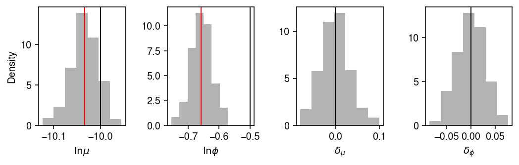
Simulate from the model.

rng = np.random.default_rng(1)
n = 500
log_mean = -10
log_inv_disp = -0.5
lam = rng.gamma(shape=np.exp(log_inv_disp), scale=np.exp(log_mean - log_inv_disp), size=2 * n)
s = 1e5
x = rng.poisson(s * lam)
z = np.zeros(2 * n, dtype=bool)
z[:n] = 1

Plot the simulated data.

cm = plt.get_cmap('Dark2')
plt.clf()
plt.gcf().set_size_inches(4, 2)
grid = np.arange(x.max() + 2)
plt.hist(x[z], bins=grid, color=cm(0), density=True, alpha=0.35)
plt.hist(x[~z], bins=grid, color=cm(1), density=True, alpha=0.25)
plt.plot(grid + .5, st.nbinom(n=np.exp(log_inv_disp), p=1 / (1 + s * np.exp(log_mean - log_inv_disp))).pmf(grid), c='k', lw=1)
plt.xlabel('Number of molecules')
plt.ylabel('Density')
plt.tight_layout()

Draw samples from the posterior.

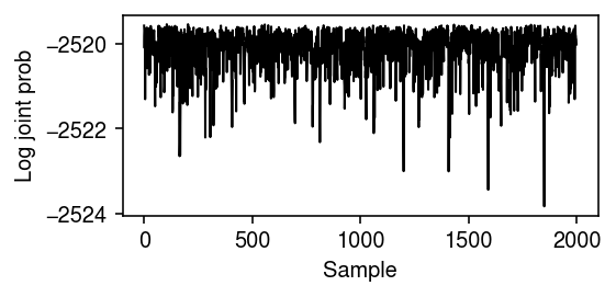
%%timeit -n1 -r1
samples, trace = diff_var_mcmc(x, s, z, n_samples=2000, trace=True)

Plot the log joint over the Markov chain.

plt.clf()
plt.gcf().set_size_inches(4, 2)
plt.plot(trace, lw=1, c='k')
plt.xlabel('Sample')
plt.ylabel('Log joint prob')
plt.tight_layout()

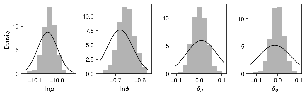
Plot the estimated posterior distribution, including reference points at the (pooled) MLE.

mle = scmodes.ebpm.ebpm_gamma(x, s)

plt.clf()
fig, ax = plt.subplots(1, 4)
fig.set_size_inches(7.5, 2.5)
for i, a in enumerate(ax):
  a.hist(samples[-500:,i], bins=7, density=True, color='0.7')
ax[0].axvline(x=log_mean, lw=1, c='k')
ax[0].axvline(x=mle[0], lw=1, c='r')
ax[1].axvline(x=log_inv_disp, lw=1, c='k')
ax[1].axvline(x=mle[1], lw=1, c='r')
ax[2].axvline(x=0, lw=1, c='k')
ax[3].axvline(x=0, lw=1, c='k')
for a in ax[:-1]:
  lim = a.get_xlim()
  grid = np.linspace(lim[0], lim[1], 1000)
ax[0].set_xlabel(r'$\ln\mu$')
ax[0].set_ylabel('Density')
ax[1].set_xlabel(r'$\ln\phi$')
ax[2].set_xlabel(r'$\delta_{\mu}$')
ax[3].set_xlabel(r'$\delta_{\phi}$')
fig.tight_layout()

Fit VI.

m = DiffVarExprModel(
  prior_log_mean=torch.distributions.Normal(loc=mle[0], scale=1.),
  prior_log_inv_disp=torch.distributions.Normal(loc=mle[1], scale=1.))
m.fit(
  torch.tensor(x.reshape(-1, 1), dtype=torch.float),
  torch.tensor(np.ones((x.shape[0], 1)) * s, dtype=torch.float),
  torch.tensor(z.reshape(-1, 1), dtype=torch.float),
  n_epochs=2000,
  n_samples=10)

DiffVarExprModel()

Compare the approximate posterior to the sampled posterior.

plt.clf()
fig, ax = plt.subplots(1, 4)
fig.set_size_inches(7.5, 2.5)
for i, a in enumerate(ax):
  a.hist(samples[-1000:,i], bins=9, density=True, color='0.7')
for k, a in zip(['log_mean', 'log_inv_disp', 'diff_mean', 'diff_inv_disp'], ax):
  lim = a.get_xlim()
  grid = np.linspace(lim[0], lim[1], 1000)
  f = st.norm(*getattr(m, k)).pdf(grid)
  a.plot(grid, f, lw=1, c='k')
ax[0].set_xlabel(r'$\ln\mu$')
ax[0].set_ylabel('Density')
ax[1].set_xlabel(r'$\ln\phi$')
ax[2].set_xlabel(r'$\delta_{\mu}$')
ax[3].set_xlabel(r'$\delta_{\phi}$')
fig.tight_layout()

Differential variance analysis

Table of Contents

Introduction

Setup

Methods

Mechanistic basis of effects on variance

Frequentist approaches to detect differential variance

Bayesian approaches to detect differential variance

Variational inference

MCMC

Data sets

STRUCTURE plot

Results

Mean-dispersion relationship

Null simulation

Fitting kinetic models directly

iPSC data

iPSC-CM time course data

Variational inference

Null simulation

DE

DD

Simulation study

Slice within Gibbs

Null example