Poisson-Beta model

Introduction
Setup
Methods
Results

Introduction

One idealized model for transcriptional regulation is the telegraph model (Peccoud and Ycart 1995, Raj et al. 2006, Kim and Marioni 2013, Munsky et al. 2013), whose steady state is described by \( \DeclareMathOperator\Bin{Binomial} \DeclareMathOperator\B{Beta} \DeclareMathOperator\Gam{Gamma} \DeclareMathOperator\Pois{Poisson} \DeclareMathOperator\betafun{B} \newcommand\E[1]{\left\langle #1 \right\rangle} \newcommand\aoff{a_{\text{off}}} \newcommand\aon{a_{\text{on}}} \newcommand\ar{a_r} \newcommand\boff{b_{\text{off}}} \newcommand\bon{b_{\text{on}}} \newcommand\br{b_r} \newcommand\const{\mathrm{const}} \newcommand\koff{k_{\text{off}}} \newcommand\kon{k_{\text{on}}} \newcommand\kr{k_r} \)

\begin{align*} x_i \mid p_i, \kr &\sim \Pois(p_i \kr)\\ p_i \mid \kon, \koff &\sim \B(\kon, \koff) \end{align*}

where \(x_i\) is the number of mRNA molecules in cell \(i=1, \ldots, n\) (considering only one gene), \(\kon\) is the rate of off\(\rightarrow\)on promoter switching, \(\koff\) is the rate of on\(\rightarrow\)off promoter switching, and \(\kr\) is the rate of mRNA synthesis. (All rates are scaled relative to the mRNA decay rate.)

The inference goal is to estimate \(\kr, \kon, \koff\) given data \(x\) assumed to be at steady state. The marginal likelihood \(p(x_i \mid \kr, \kon, \koff)\) does have a closed form; however, it involves the confluent hypergeometric function of the first kind (Raj et al 2006), which is difficult to evaluate. To avoid this challenge, Kim and Marioni 2013 develop an MCMC scheme to sample from the posterior \(p(\kr, \kon, \koff \mid x_1, \ldots, x_n)\), and Larsson et al. 2019 use numerical integration to evaluate the marginal likelihood.

We collected these different inference algorithms into a Python package poisbeta. Here, we investigate how the running time of the MLE procedure (using numerical integration) scales, and whether variational inference can improve the running time. We also investigate the effect of size factors (Kim and Marioni 2013) and initialization on the estimates.

Setup

import colorcet
import itertools as it
import numpy as np
import pandas as pd
import poisbeta
import scmodes
import scipy.optimize as so
import scipy.special as sp
import scipy.stats as st
import sys
import timeit

%matplotlib inline
%config InlineBackend.figure_formats = set(['retina'])

import matplotlib.pyplot as plt
plt.rcParams['figure.facecolor'] = 'w'
plt.rcParams['font.family'] = 'Nimbus Sans'

Methods

Moment estimation

Peccoud and Ycart 1995 derived moment estimators for \(\kr, \kon, \koff\)

def fit_poisson_beta_moment(x, **kwargs):
  """Return ln kr, ln kon, ln koff

  Estimate kr, kon, koff using the first three exponential moments (Peccoud &
  Ycart 1995).

  x - array-like [n,]

  """
  moments = np.array([1, x.mean(), (x * (x - 1)).mean(), (x * (x - 1) * (x - 2)).mean()])
  ratios = moments[1:] / moments[:-1]
  kr = (2 * ratios[0] * ratios[2] - ratios[0] * ratios[1] - ratios[1] * ratios[2]) / (ratios[0] - 2 * ratios[1] + ratios[2])
  kon = (2 * ratios[0] * (ratios[2] - ratios[1])) / (ratios[0] * ratios[1] - 2 * ratios[0] * ratios[2] + ratios[1] * ratios[2])
  koff = (2 * (ratios[2] - ratios[1]) * (ratios[0] - ratios[2]) * (ratios[1] - ratios[0])) / ((ratios[0] * ratios[1] - 2 * ratios[0] * ratios[2] + ratios[1] * ratios[2]) * (ratios[0] - 2 * ratios[1] + ratios[2]))
  result = np.array([kr, kon, koff])
  if not (np.isfinite(result).all() and (result > 0).all()):
    raise RuntimeError('moment estimation failed')
  return np.log(result)

Maximum likelihood estimation

Larsson et al. 2019 use Gauss-Jacobi quadrature to evaluate the marginal likelihood

\begin{align*} \ell &= \frac{1}{\betafun(\kon, \koff)} \int_0^1 \Pois(x_i; \kr p_i)\, p_i^{\kon - 1} (1 - p_i)^{\koff - 1}\; dp_i\\ &= \frac{1}{2^{\kon + \koff - 1} \betafun(\kon, \koff)} \int_{-1}^1 \Pois(x_i; \kr \frac{1 + t_i}{2})\, (1 + t_i)^{\kon - 1} (1 - t_i)^{\koff - 1}\; dt_i\\ &\approx \frac{1}{2^{\kon + \koff - 1} \betafun(\kon, \koff)} \sum_{k=1}^K w_k \Pois(x_i; \kr y_k) \end{align*}

where \(\betafun(\cdot)\) denotes the Beta function, \(y_k\) is the root of the Jacobi polynomial of degree \(k\), and \(w_k\) is the associated weight. This procedure can be used as a subroutine to numerically optimize the marginal likelihood.

Slice-within-Gibbs sampling

Kim & Marioni 2013 add priors

\begin{align*} \kr \mid \ar, \br &\sim \Gam(\ar, \br)\\ \kon \mid \aon, \bon &\sim \Gam(\aon, \bon)\\ \koff \mid \aoff, \boff &\sim \Gam(\aoff, \boff) \end{align*}

The conditional (log) densities are available, up to constants

\begin{align*} \ln p(p_i \mid \cdot) &= (x_i + \kon - 1) \ln p_i + (\koff - 1)\ln(1 - p_i) - \kr p_i + \const\\ \ln p(\kr \mid \cdot) &= \sum_i [(x_i + \ar - 1) \ln \kr - (p_i + \br) \kr] + \const\\ \ln p(\kon \mid \cdot) &= \sum_i [\kon \ln p_i + (\aon - 1)\ln \kon - \bon\kon - \ln\Gamma(\kon) + \ln\Gamma(\kon + \koff)] + \const\\ \ln p(\koff \mid \cdot) &= \sum_i [\koff \ln (1 - p_i) + (\aoff - 1)\ln \koff - \boff\koff - \ln\Gamma(\koff) + \ln\Gamma(\kon + \koff)] + \const \end{align*}

Although the conditional distributions are non-standard, slice sampling (Neal 2003) only requires the target density up to a constant.

Variational inference

To make the model amenable for VI, introduce latent variables \(z_i\)

\begin{align*} x_i \mid z_i, p_i &\sim \Bin(z_i, p_i)\\ z_i \mid \kr &\sim \Pois(\kr)\\ p_i \mid \kon, \koff &\sim \B(\kon, \koff) \end{align*}

Then, we have

\begin{multline*} \ln p(x_i, z_i, p_i \mid \kr, \kon, \koff) = (x + \kon - 1) \ln p_i + (z_i - x_i + \koff - 1) \ln(1 - p_i)\\ + (z_i - x_i) \ln \kr - \kr + x_i \ln \kr - \ln\Gamma(x_i + 1) - \ln\Gamma(z_i - x_i + 1) - \ln\betafun(\kon, \koff) \end{multline*}

where we have added and subtracted \(x_i \ln \kr\) to more easily derive coordinate updates

\begin{align*} q^*(z_i - x_i) &= \Pois(\exp(\E{\ln (1 - p_i)} + \ln k_r)) \triangleq \Pois(\mu_i) \\ q^*(p_i) &= \B(x_i + \kon, \E{z_i - x_i} + \koff) \triangleq \B(\alpha_i, \beta_i) \end{align*}

where expectations are taken with respect to the variational approximation \(q\). Using properties of the Beta distribution

\begin{align*} \E{\ln p_i} &= \psi(\alpha_i) - \psi(\alpha_i + \beta_i)\\ \E{\ln (1 - p_i)} &= \psi(\beta_i) - \psi(\alpha_i + \beta_i) \end{align*}

where \(\psi\) is the digamma function. The evidence lower bound is

\begin{multline*} \ell = \sum_i (x_i + \kon - \alpha_i) \E{\ln p_i} + (\mu_i + \koff - \beta_i) \E{\ln(1 - p_i)}\\ + (x_i + \mu_i) \ln \kr - k_r - \mu_i \ln \mu_i + \mu_i - \ln\Gamma(x_i + 1) - \ln\betafun(\kon, \koff) + \ln\betafun(\alpha_i, \beta_i) \end{multline*}

We can derive the Jacobian with respect to \(\kr, \kon, \koff\), leading to an analytic update for \(\kr\). We can use Brent’s method to numerically update \(\kon, \koff\).

\begin{align*} \frac{\partial \ell}{\partial \kr} &= \sum_i \frac{x_i + \mu_i}{\kr} - 1\\ \kr &:= \frac{1}{n} \sum_i x_i + \mu_i\\ \frac{\partial \ell}{\partial \kon} &= \sum_i \psi(\alpha_i) - \psi(\alpha_i - \beta_i) - \psi(\kon) + \psi(\kon + \koff)\\ \frac{\partial \ell}{\partial \koff} &= \sum_i \psi(\beta_i) - \psi(\alpha_i - \beta_i) - \psi(\koff) + \psi(\kon + \koff) \end{align*}

Identifiability

Kim and Marioni 2013 discuss an identifiability problem with the model, which was also investigated by Orlova 2019.

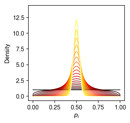
First, if \(\kon\) and \(\koff\) are large, then none of the parameters are identifiable. Specifically, for some fixed \(\kr\), taking \(\kon \rightarrow \infty\) and \(\koff \rightarrow \infty\), we have \(p_i \sim \delta(p_i - 0.5)\).

grid = np.linspace(0, 1, 1000)
plt.clf()
plt.gcf().set_size_inches(3, 3)
a_max = 5
for a in np.linspace(0, a_max, 20):
  plt.plot(grid, st.beta(a=np.exp(a), b=np.exp(a)).pdf(grid), lw=1, c=colorcet.cm['fire'](a / a_max))
plt.xlabel('$p_i$')
plt.ylabel('Density')
plt.tight_layout()

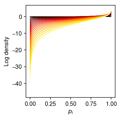
But if we take \(\kon \rightarrow \infty\) and \(\koff \rightarrow 0\), we get \(p_i \sim \delta(p_i - 1)\), and we could achieve the same likelihood by scaling \(\kr / 2\).

grid = np.linspace(0, 1, 1000)
plt.clf()
plt.gcf().set_size_inches(3, 3)
a_max = 2
for a in np.linspace(0, a_max, 20):
  plt.plot(grid, st.beta(a=np.exp(a), b=np.exp(-a)).logpdf(grid), lw=1, c=colorcet.cm['fire'](a / a_max))
plt.xlabel('$p_i$')
plt.ylabel('Log density')
plt.tight_layout()

Second, if \(\koff\) is large, then \(\koff\) and \(\kr\) are unidentifiable. Holding \(\kon\) fixed, we have \(E[p_i] = \kon / (\kon + \koff)\), and intuitively we can achieve the same likelihood by taking \(\kr \rightarrow \infty\) as \(\koff \rightarrow \infty\).

There are two ways we could address this prolblem:

Reparametrize the model: Let \(\gamma\) be the average length of the on/off cycle, and \(\delta\) be the average ratio of time spent in the on versus off state during that cycle. Then, we have
\begin{align*} \delta &= \frac{1 / \kon}{1 / \koff} = \frac{\koff}{\kon}\\ \gamma &= \frac{1}{1 / \kon + 1 / \koff} = \frac{\kon\koff}{\kon + \koff}\\ \kon &= \frac{\gamma(\delta + 1)}{\delta}\\ \koff &= \gamma(\delta + 1) \end{align*}
This parametrization still implicitly scales time relative to the mRNA decay rate, and implies e.g. \(E[x_i] = \kr/(1 + \delta)\). However, it suggests very different priors
\begin{align*} \gamma &\sim \operatorname{Exponential}(1/\mu)\\ \delta &\sim \operatorname{Uniform}(0, 1) \end{align*}
We can use this parametrization in slice-within-Gibbs:
\begin{align*} \ln p(\gamma \mid \cdot) &= \sum_i \left(\frac{\gamma(\delta + 1)}{\delta}\right) \ln p_i + \gamma(\delta + 1) \ln (1 - p_i) - \ln \betafun\left(\frac{\gamma(\delta + 1)}{\delta}, \gamma(\delta + 1)\right) - \frac{\gamma}{\mu} + \const\\ \ln p(\delta \mid \cdot) &= \sum_i \left(\frac{\gamma(\delta + 1)}{\delta}\right) \ln p_i + \gamma(\delta + 1) \ln (1 - p_i) + \const \end{align*}
Use informative priors: Larsson et al. 2019 collected data on mRNA decay rates.

Simulation

Draw data from the basic model.

def simulate_pois_beta(n, s=None, kr=None, kon=None, koff=None, seed=None):
  if seed is not None:
    np.random.seed(seed)
  if kr is None:
    kr = np.random.lognormal(mean=3)
  if kon is None:
    kon = np.random.lognormal()
  if koff is None:
    koff = np.random.lognormal()
  if s is None:
    s = 1
  p = np.random.beta(a=kon, b=koff, size=n)
  x = np.random.poisson(lam=s * kr * p)
  return x, kr, kon, koff

Draw data from a model with size factors.

\begin{align*} x_i \mid s_i, p_i, \kr &\sim \Pois(s_i p_i \kr)\\ p_i \mid \kon, \koff &\sim \B(\kon, \koff) \end{align*}

def trial(n, mean_size, var_size, kr, kon, koff, seed):
  np.random.seed(seed)
  disp = (var_size - mean_size) / (mean_size * mean_size)
  s = np.random.poisson(lam=mean_size, size=n) * np.random.gamma(shape=1 / disp, scale=disp, size=n)
  x, *theta = simulate_pois_beta(n=n, s=s, kr=kr / mean_size, kon=kon, koff=koff, seed=1)
  theta0 = fit_poisson_beta_moment(x)
  theta0[0] -= np.log(s).mean()
  theta1 = fit_poisson_beta_mle(x)
  theta1[0] -= np.log(s).mean()
  theta2 = fit_poisson_beta_mle(x, s, init=theta0)
  return x, s, [np.log(theta), theta0, theta1, theta2]

Results

Simulation

Make sure the implementations work on one example.

x, *theta = simulate_pois_beta(n=1000, seed=0)
theta

[117.2199806492514, 1.4920592434019648, 2.661095776728801]

Fit the moment estimator.

thetahat_moment = fit_poisson_beta_moment(x)
np.exp(thetahat_moment)

array([120.04495743,   1.52142758,   2.72068022])

Fit the MLE.

thetahat_mle = fit_poisson_beta_mle(x)
np.exp(thetahat_mle)

array([118.92485772,   1.52953485,   2.68994176])

Evaluate more systematically.

def evaluate_estimator(n, n_trials):
  sim_result = []
  grid = np.linspace(np.log(.1), np.log(100), 5)
  for (ln_kr, ln_kon, ln_koff) in itertools.product(grid, repeat=3):
    for trial in range(n_trials):
      x, *_ = simulate_pois_beta(n=n, kr=np.exp(ln_kr), kon=np.exp(ln_kon),
                                 koff=np.exp(ln_koff), seed=trial)
      for method in ['moment', 'mle']:
        try:
          thetahat = getattr(sys.modules['__main__'], f'fit_poisson_beta_{method}')(x)
        except RuntimeError:
          thetahat = [np.nan, np.nan, np.nan]
        sim_result.append([ln_kr, ln_kon, ln_koff, method, trial] + list(thetahat))
  return pd.DataFrame(sim_result, columns=['ln_kr', 'ln_kon', 'ln_koff', 'method', 'trial', 'ln_kr_hat', 'ln_kon_hat', 'ln_koff_hat'])

res = evaluate_estimator(n=100, n_trials=1)

Report the fraction of data sets for which estimation failed.

res.groupby(['method']).apply(lambda x: x.dropna().shape[0] / x.shape[0])

method
mle       0.584
moment    0.296
dtype: float64

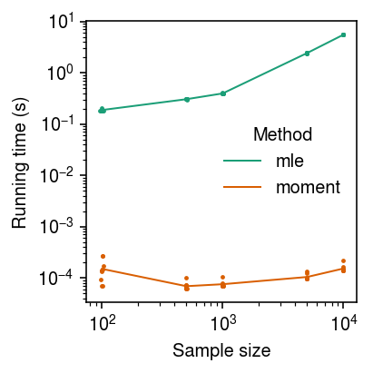
Running time benchmark

def evaluate_running_time(n_trials):
  timing_result = []
  for n in (100, 500, 1000, 5000, 10000):
    # Fix the parameters to something easy
    x, *_ = simulate_pois_beta(n=n, kr=50, kon=1, koff=1, seed=0)
    for m in ('moment', 'mle'):
      res = timeit.repeat(stmt=lambda: getattr(sys.modules['__main__'], f'fit_poisson_beta_{m}')(x),
                          number=1, repeat=n_trials, globals=locals())
      for i, t in enumerate(res):
        timing_result.append([n, m, i, t])
  return pd.DataFrame(timing_result, columns=['n', 'method', 'trial', 'time'])

timing_res = evaluate_running_time(n_trials=10)

cm = plt.get_cmap('Dark2')
plt.clf()
plt.gcf().set_size_inches(3, 3)
plt.xscale('log')
plt.yscale('log')
for i, (m, g) in enumerate(timing_res.groupby('method')):
  t = g.groupby('n')['time'].agg([np.mean, np.std]).reset_index()
  plt.plot(t['n'], t['mean'], lw=1, c=cm(i), label=m)
  plt.scatter(g['n'] + np.random.normal(scale=np.log10(g['n']), size=g.shape[0]), g['time'], c=cm(i), s=2, label=None)
plt.legend(frameon=False, title='Method')
plt.xlabel('Sample size')
plt.ylabel('Running time (s)')
plt.tight_layout()

Impact of size factors

Simulate a simple example with non-trivial size factor variation. Plot the estimated distributions, as well as the difference between the fitted Beta distributions and the ground truth.

x, s, res = trial(n=1000, mean_size=10000, var_size=250000, kr=32, kon=.5, koff=.25, seed=0)

cm = plt.get_cmap('Dark2')
plt.clf()
fig, ax = plt.subplots(2, 1)
fig.set_size_inches(6, 4)

grid = np.arange(x.max() + 1)
ax[0].hist(x, bins=grid, color='0.5')

for i, (log_theta, label) in enumerate(zip(res, ['Ground truth', 'Moment', 'MLE (posthoc)', 'MLE'])):
  p = np.array([poisson_beta_pmf(log_theta, i, s).mean() for i in grid[:-1]])
  ax[0].plot(.5 + grid[:-1], n * p, lw=1, c=cm(i), label=label)
ax[0].legend(frameon=False, bbox_to_anchor=(1, .5), loc='center left')
ax[0].set_xlabel('Number of molecules')
ax[0].set_ylabel('Number of cells')

grid = np.linspace(0, 1, 1000)
fp = st.beta(a=kon, b=koff).logpdf(grid)
for i, (log_theta, label) in enumerate(zip(res, ['Ground truth', 'Moment', 'MLE (posthoc)', 'MLE'])):
  if i > 0:
    ax[1].plot(grid, fp - st.beta(a=np.exp(log_theta[1]), b=np.exp(log_theta[2])).logpdf(grid), lw=1, c=cm(i))
ax[1].axhline(y=0, lw=1, ls=':', c='k')
ax[1].set_xlabel('$p_i$')
ax[1].set_ylabel('Diff log density\nfrom ground truth')

fig.tight_layout()

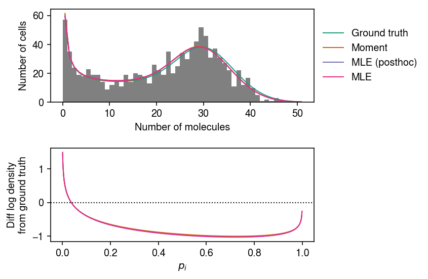
Compare the log likelihoods of the fitted models.

pd.Series({k: poisson_beta_neg_llik(log_theta, x, s) for k, log_theta 
           in zip(['ground_truth', 'moment', 'mle_poshoc', 'mle'], res)})

ground_truth    3692.394156
moment          3690.490051
mle_poshoc      3690.382941
mle             3690.376902
dtype: float64

Look at some more examples.

x, s, res = trial(n=int(1e3), mean_size=1e5, var_size=4e5, kr=64, kon=2, koff=.5, seed=1)

cm = plt.get_cmap('Dark2')
plt.clf()
fig, ax = plt.subplots(2, 1)
fig.set_size_inches(6, 4)

grid = np.arange(x.max() + 1)
ax[0].hist(x, bins=grid, color='0.5')

for i, (log_theta, label) in enumerate(zip(res, ['Ground truth', 'Moment', 'MLE (posthoc)', 'MLE'])):
  p = np.array([poisson_beta_pmf(log_theta, i, s).mean() for i in grid[:-1]])
  ax[0].plot(.5 + grid[:-1], n * p, lw=1, c=cm(i), label=label)
ax[0].legend(frameon=False, bbox_to_anchor=(1, .5), loc='center left')
ax[0].set_xlabel('Number of molecules')
ax[0].set_ylabel('Number of cells')

grid = np.linspace(0, 1, 1000)
fp = st.beta(a=kon, b=koff).logpdf(grid)
for i, (log_theta, label) in enumerate(zip(res, ['Ground truth', 'Moment', 'MLE (posthoc)', 'MLE'])):
  if i > 0:
    ax[1].plot(grid, fp - st.beta(a=np.exp(log_theta[1]), b=np.exp(log_theta[2])).logpdf(grid), lw=1, c=cm(i))
ax[1].set_xlabel('$p_i$')
ax[1].set_ylabel('Diff log density\nfrom ground truth')

fig.tight_layout()

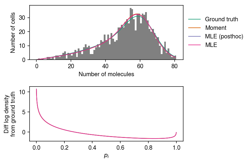
pd.Series({k: poisson_beta_neg_llik(log_theta, x, s) for k, log_theta 
           in zip(['ground_truth', 'moment', 'mle_poshoc', 'mle'], res)})

ground_truth    4053.912218
moment          4052.601052
mle_poshoc      4052.557805
mle             4052.557227
dtype: float64

Log likelihood surface

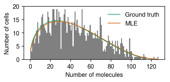
Simulate a single example.

x, *theta = simulate_pois_beta(n=1000, seed=0)
log_theta = np.log(np.array(theta))
log_theta_hat = fit_poisson_beta_mle(x)

Plot the simulated data.

cm = plt.get_cmap('Dark2')
plt.clf()
plt.gcf().set_size_inches(4, 2)
grid = np.arange(x.max() + 1)
plt.hist(x, bins=grid, color='0.5')
for i, (k, v) in enumerate(zip(['Ground truth', 'MLE'], [log_theta, log_theta_hat])):
  p = np.array([poisson_beta_pmf(v, i, 1).mean() for i in grid[:-1]])
  plt.plot(.5 + grid[:-1], 1000 * p, lw=1, c=cm(i), label=k)
plt.legend(frameon=False)
plt.xlabel('Number of molecules')
plt.ylabel('Number of cells')
plt.tight_layout()

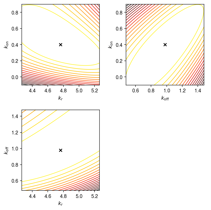
Draw the log likelihood surface about the true value.

M = 100
grid_kr = np.linspace(log_theta[0] - .5, log_theta[0] + .5, M)
grid_kon = np.linspace(log_theta[1] - .5, log_theta[1] + .5, M)
grid_koff = np.linspace(log_theta[2] - .5, log_theta[2] + .5, M)

llik_kr_kon = np.zeros((M, M))
for i in range(M):
  for j in range(M):
    llik_kr_kon[i, j] = poisson_beta_neg_llik(np.array([grid_kr[i], grid_kon[j], log_theta[2]]), x, 1)

llik_kr_koff = np.zeros((M, M))
for i in range(M):
  for j in range(M):
    llik_kr_koff[i, j] = poisson_beta_neg_llik(np.array([grid_kr[i], log_theta[1], grid_koff[j]]), x, 1)

llik_kon_koff = np.zeros((M, M))
for i in range(M):
  for j in range(M):
    llik_kon_koff[i, j] = poisson_beta_neg_llik(np.array([log_theta[0], grid_kon[i], grid_koff[j]]), x, 1)

cm = colorcet.cm['fire_r']
plt.clf()
fig, ax = plt.subplots(2, 2)
fig.set_size_inches(6, 6)

ax[0,0].contour(grid_kr, grid_kon, llik_kr_kon, cmap=cm, linewidths=1, levels=np.linspace(llik_kr_kon.min(), llik_kr_kon.max(), 20))
ax[0,0].scatter(log_theta[0], log_theta[1], marker='x', s=32, c='k', label='Ground truth')
ax[0,0].scatter(log_theta_hat[0], log_theta_hat[1], marker='x', s=32, c='r', label='MLE')
ax[0,0].legend(handletextpad=0)
ax[0,0].set_xlabel('$\ln(k_r)$')
ax[0,0].set_ylabel('$\ln(k_{\mathrm{on}})$')

ax[1,0].contour(grid_kr, grid_koff, llik_kr_koff, cmap=cm, levels=np.linspace(llik_kr_koff.min(), llik_kr_koff.max(), 20), linewidths=1)
ax[1,0].scatter(log_theta[0], log_theta[2], marker='x', s=32, c='k')
ax[1,0].scatter(log_theta_hat[0], log_theta_hat[2], marker='x', s=32, c='r')
ax[1,0].set_xlabel('$\ln(k_r)$')
ax[1,0].set_ylabel('$\ln(k_{\mathrm{off}})$')

ax[0,1].contour(grid_koff, grid_kon, llik_kon_koff.T, cmap=cm, levels=np.linspace(llik_kon_koff.min(), llik_kon_koff.max(), 20), linewidths=1)
ax[0,1].scatter(log_theta[2], log_theta[1], marker='x', s=32, c='k')
ax[0,1].scatter(log_theta_hat[2], log_theta_hat[1], marker='x', s=32, c='r')
ax[0,1].set_xlabel('$\ln(k_{\mathrm{off}})$')
ax[0,1].set_ylabel('$\ln(k_{\mathrm{on}})$')

ax[1,1].set_axis_off()

fig.tight_layout()

Impact of initialization

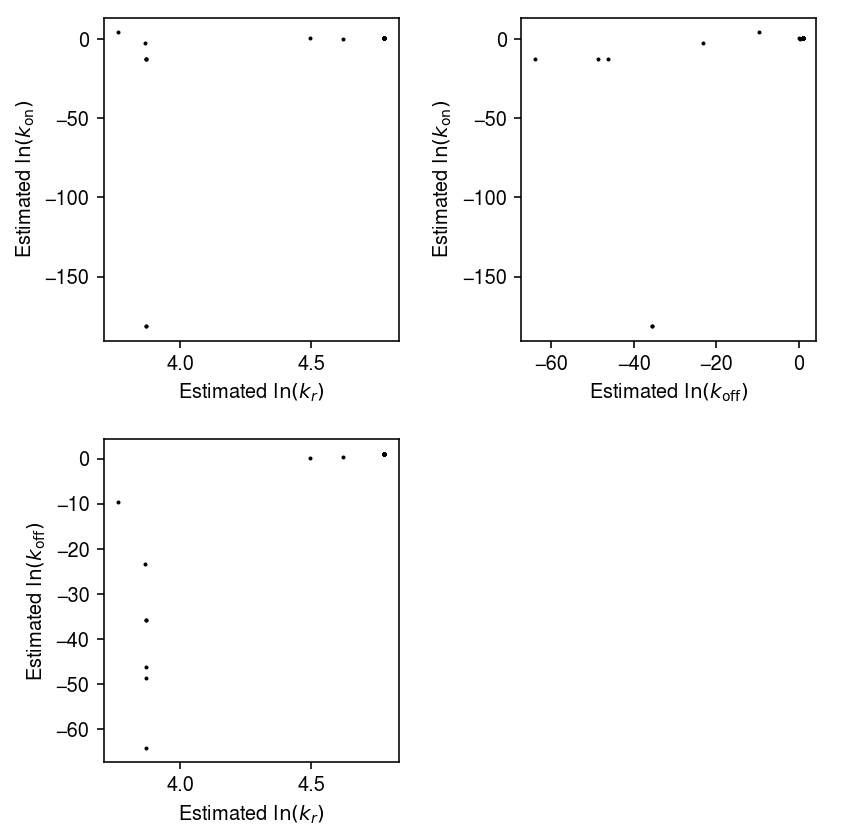
Look at estimates starting from random initializations.

thetahat = []
for i in range(100):
  try:
    res = fit_poisson_beta_mle(x, init=np.random.normal(scale=0.5, size=3), max_iters=10000)
  except RuntimeError as e:
    print(f'Initialization {i} failed: {e.__cause__}')
  if not i % 10:
    print(f'Trial {i}')
  thetahat.append(res)
thetahat = np.array(thetahat)

plt.clf()
fig, ax = plt.subplots(2, 2)
fig.set_size_inches(6, 6)
ax[0,0].scatter(thetahat[:,0], thetahat[:,1], s=1, c='k')
ax[0,0].set_xlabel('Estimated $\ln(k_r)$')
ax[0,0].set_ylabel('Estimated $\ln(k_{\mathrm{on}})$')

ax[1,0].scatter(thetahat[:,0], thetahat[:,2], s=1, c='k')
ax[1,0].set_xlabel('Estimated $\ln(k_r)$')
ax[1,0].set_ylabel('Estimated $\ln(k_{\mathrm{off}})$')

ax[0,1].scatter(thetahat[:,2], thetahat[:,1], s=1, c='k')
ax[0,1].set_xlabel('Estimated $\ln(k_{\mathrm{off}})$')
ax[0,1].set_ylabel('Estimated $\ln(k_{\mathrm{on}})$')

ax[1,1].set_axis_off()
fig.tight_layout()

(pd.DataFrame(thetahat, columns=['log_kr', 'log_kon', 'log_koff'])
 .to_csv('/scratch/midway2/aksarkar/ideas/poisson-beta-est.txt.gz', sep='\t'))

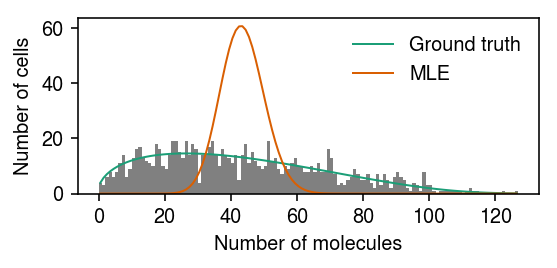
Look at one example where the fit converged to something far from the ground truth.

query = thetahat[np.argmin(thetahat[:,0])]

cm = plt.get_cmap('Dark2')
plt.clf()
plt.gcf().set_size_inches(4, 2)
grid = np.arange(x.max() + 1)
plt.hist(x, bins=grid, color='0.5')
for i, (k, v) in enumerate(zip(['Ground truth', 'MLE'], [log_theta, query])):
  p = np.array([poisson_beta_pmf(v, i, 1).mean() for i in grid[:-1]])
  plt.plot(.5 + grid[:-1], 1000 * p, lw=1, c=cm(i), label=k)
plt.legend(frameon=False)
plt.xlabel('Number of molecules')
plt.ylabel('Number of cells')
plt.tight_layout()

Slice-within-Gibbs sampling

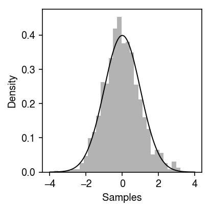
First, try to sample from a standard Gaussian using slice sampling.

import poisbeta.mcmc
f = st.norm().logpdf
n_samples = 1000
samples = [0]
for i in range(n_samples):
  x = poisbeta.mcmc.slice_sample(f, width=5, init=samples[-1])
  samples.append(x)
samples = np.array(samples[1:])

grid = np.linspace(-4, 4, 1000)
plt.clf()
plt.gcf().set_size_inches(3, 3)
plt.hist(samples, bins=30, density=True, color='0.7')
plt.plot(grid, np.exp(f(grid)), lw=1, c='k')
plt.xlabel('Samples')
plt.ylabel('Density')
plt.tight_layout()

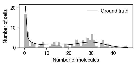
Now, simulate a simple data set.

x, *theta = simulate_pois_beta(n=100, kr=32, kon=.25, koff=.25, seed=0)
log_theta = np.log(np.array(theta))

grid = np.arange(x.max() + 1)
n = x.shape[0] * np.array([poisbeta.mle.poisson_beta_pmf(log_theta, i, 1) for i in grid]).ravel()
plt.clf()
plt.gcf().set_size_inches(4, 2)
plt.hist(x, bins=grid, color='0.7')
plt.plot(grid + 0.5, n, lw=1, c='k', label='Ground truth')
plt.legend(frameon=False)
plt.xlabel('Number of molecules')
plt.ylabel('Number of cells')
plt.tight_layout()

Use slice-within-Gibbs to sample from the posterior \(p(\kr, \kon, \koff \mid x_1, \ldots, x_n)\).

# Important: Kim & Marioni 2013 use shape/scale parametrization, but write
# alpha/beta. We use shape/rate
samples, trace = poisbeta.mcmc.fit_poisson_beta_mcmc(
  x,
  n_samples=1000,
  ar=1,
  br=1/x.max(),
  aon=1,
  bon=1/100,
  aoff=1,
  boff=1/100,
  trace=True)

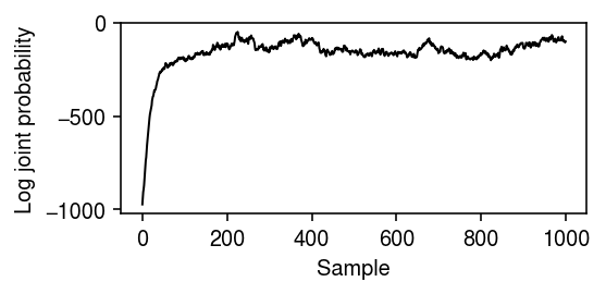
Plot the evolution of the log joint probability over the samples.

plt.clf()
plt.gcf().set_size_inches(4, 2)
plt.plot(np.arange(samples.shape[0]), trace, lw=1, c='k')
plt.xlabel('Sample')
plt.ylabel('Log joint probability')
plt.tight_layout()

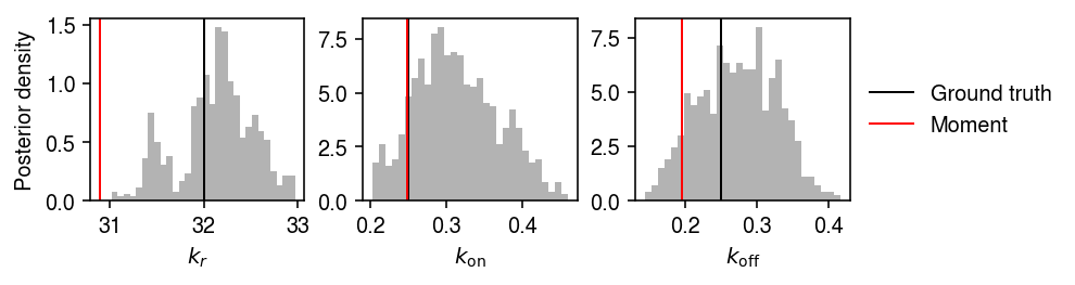
Look at the posterior distributions over the parameters. Use 800 samples after warm-up, based on the evolution of the log joint probability. Superimpose the moment estimate.

thetahat = np.exp(poisbeta.fit_poisson_beta_moment(x))

plt.clf()
fig, ax = plt.subplots(1, 3)
fig.set_size_inches(7, 2)
for a, s, t, h, k in zip(ax, samples.T, theta, thetahat, ['$k_r$', '$k_{\mathrm{on}}$', '$k_{\mathrm{off}}$']):
  a.hist(s[-800:], bins=30, density=True, color='0.7')
  a.axvline(x=t, c='k', lw=1, label='Ground truth')
  a.axvline(x=h, c='r', lw=1, label='Moment')
  a.set_xlabel(k)
ax[0].set_ylabel('Posterior density')
ax[-1].legend(frameon=False, loc='center left', bbox_to_anchor=(1, .5))
fig.tight_layout()

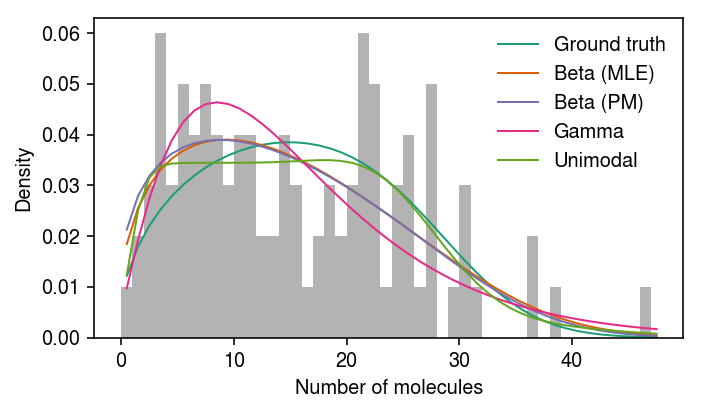
Kim and Marioni discuss an identifiability problem with the model. Simulate an example data set. Estimate the MLE, and draw samples from the posterior of the Poisson-Beta model. Then, fit a Gamma assumption and a unimodal assumption on expression variation.

x, *theta = simulate_pois_beta(n=100, kr=32, kon=1.5, koff=1.5, seed=0)

samples, trace = poisbeta.mcmc.fit_poisson_beta_mcmc(
  x,
  n_samples=1000,
  ar=1,
  br=1/x.max(),
  aon=1,
  bon=1/100,
  aoff=1,
  boff=1/100,
  trace=True)

ebpm_beta_res = poisbeta.fit_poisson_beta_mle(x)
ebpm_gamma_res = scmodes.ebpm.ebpm_gamma(x, 1)
ebpm_unimodal_res = scmodes.ebpm.ebpm_unimodal(x, 1)

Report the log likelihoods achieved by the point estimates.

pd.Series({
  'beta': poisbeta.mle.poisson_beta_logpmf(thetahat, x, 1).sum(),
  'gamma': ebpm_gamma_res[-1],
  'unimodal': np.array(ebpm_unimodal_res.rx2('loglik'))[0],
})

beta       -371.722956
gamma      -363.271122
unimodal   -359.050396
dtype: float64

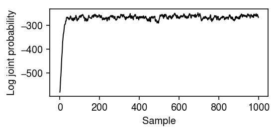
Plot the MCMC trace.

plt.clf()
plt.gcf().set_size_inches(4, 2)
plt.plot(np.arange(samples.shape[0]), trace, lw=1, c='k')
plt.xlabel('Sample')
plt.ylabel('Log joint probability')
plt.tight_layout()

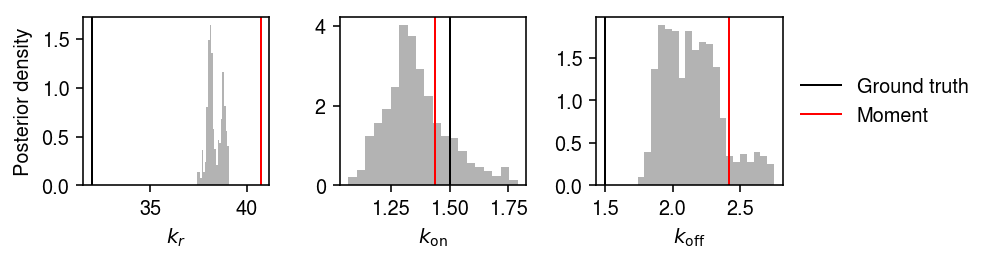
Plot the estimated posteriors and the point estimates.

plt.clf()
fig, ax = plt.subplots(1, 3)
fig.set_size_inches(7, 2)
for a, s, t, h, k in zip(ax, samples.T, theta, np.exp(ebpm_beta_res), ['$k_r$', '$k_{\mathrm{on}}$', '$k_{\mathrm{off}}$']):
  a.hist(s[-800:], bins=20, density=True, color='0.7')
  a.axvline(x=t, c='k', lw=1, label='Ground truth')
  a.axvline(x=h, c='r', lw=1, label='Moment')
  a.set_xlabel(k)
ax[0].set_ylabel('Posterior density')
ax[-1].legend(frameon=False, loc='center left', bbox_to_anchor=(1, .5))
fig.tight_layout()

Plot the simulated data and estimated distributions.

cm = plt.get_cmap('Dark2')
grid = np.arange(x.max() + 1)
plt.clf()
plt.gcf().set_size_inches(5, 3)
plt.hist(x, bins=grid, density=True, color='0.7')

plt.plot(grid + 0.5, np.array([poisbeta.mle.poisson_beta_pmf(np.log(np.array(theta)), i, 1) for i in grid]).ravel(), lw=1, c=cm(0), label='Ground truth')

plt.plot(grid + 0.5, np.array([poisbeta.mle.poisson_beta_pmf(ebpm_beta_res, i, 1) for i in grid]).ravel(), lw=1, c=cm(1), label='Beta (MLE)')

pm = np.log(samples[-800:]).mean(axis=0)
plt.plot(grid + 0.5, np.array([poisbeta.mle.poisson_beta_pmf(pm, i, 1) for i in grid]).ravel(), lw=1, c=cm(2), label='Beta (PM)')

plt.plot(grid + 0.5, st.nbinom(n=np.exp(ebpm_gamma_res[1]), p=1 / (1 + np.exp(ebpm_gamma_res[0] - ebpm_gamma_res[1]))).pmf(grid), lw=1, c=cm(3), label='Gamma')

g = np.array(ebpm_unimodal_res.rx2('fitted_g'))
a = np.fmin(g[1], g[2])
b = np.fmax(g[1], g[2])
comp_dens_conv = np.array([((st.gamma(a=k + 1, scale=1).cdf(b.reshape(1, -1)) - st.gamma(a=k + 1, scale=1).cdf(a.reshape(1, -1))) / (b - a)).mean(axis=0) for k in grid])
comp_dens_conv[:,0] = st.poisson(mu=b[0]).pmf(x).mean(axis=0)
plt.plot(grid + 0.5, comp_dens_conv @ g[0], lw=1, c=cm(4), label='Unimodal')

plt.legend(frameon=False)
plt.xlabel('Number of molecules')
plt.ylabel('Density')
plt.tight_layout()

Poisson-Beta model

Table of Contents

Introduction

Setup

Methods

Moment estimation

Maximum likelihood estimation

Slice-within-Gibbs sampling

Variational inference

Identifiability

Simulation

Results

Simulation

Running time benchmark

Impact of size factors

Log likelihood surface

Impact of initialization

Slice-within-Gibbs sampling