Weighted negative binomial matrix factorization
Table of Contents
Introduction
Negative Binomial Matrix Factorization (NBMF; Gouvert et al 2018) is the (augmented) model \( \newcommand\const{\mathrm{const}} \newcommand\E[1]{\left\langle #1 \right\rangle} \newcommand\vx{\mathbf{x}} \newcommand\vw{\mathbf{w}} \newcommand\vz{\mathbf{z}} \newcommand\mx{\mathbf{X}} \newcommand\mU{\mathbf{U}} \newcommand\mw{\mathbf{W}} \newcommand\mz{\mathbf{Z}} \newcommand\ml{\mathbf{L}} \newcommand\mf{\mathbf{F}} \)
\begin{align*} x_{ij} &= \sum_{k=1}^K z_{ijk}\\ z_{ijk} &\sim \operatorname{Poisson}(l_{ik} f_{jk} u_{ij})\\ u_{ij} &\sim \operatorname{Gamma}(1/\phi_{ij}, 1/\phi_{ij}) \end{align*}where the Gamma distribution is parameterized by a shape and a rate. (The mean of the Gamma distribution is 1, and its variance is \(\phi_{ij}\).) Gouvert et al. 2018 only consider the case \(\phi_{ij} = \phi\); however, other natural choices are \(\phi_{ij} = \phi_j\) and \(\phi_{ij} = \phi_i \phi_j\). The model admits analytic EM updates for \(\ml\) and \(\mf\), and numerical updates for the simple case \(\phi_{ij} = \phi\).
Here, we study the imputation performance of WNBMF on simulated problems.
Setup
import itertools as it
import numpy as np
import pandas as pd
import scipy.stats as st
import scmodes
%matplotlib inline
%config InlineBackend.figure_formats = set(['retina'])
import matplotlib.pyplot as plt
plt.rcParams['figure.facecolor'] = 'w'
plt.rcParams['font.family'] = 'Nimbus Sans'
Methods
Simulation
Draw data from the model, assuming \(\phi_{ij} = \phi\). We define "proportion of variance explained" as \(\operatorname{Var}(\mu_{ij}) / (\operatorname{Var}(\mu_{ij}) + \operatorname{Var}(u_{ij}))\).
def simulate(n, p, k, pve=0.5, seed=0, mu_max=None):
  np.random.seed(seed)
  l = np.random.lognormal(sigma=.5, size=(n, k))
  f = np.random.lognormal(sigma=.5, size=(p, k))
  mu = l.dot(f.T)
  if mu_max is not None:
    mu *= mu_max / mu.max()
  if pve < 1:
    inv_disp = 1 / ((1 / pve - 1) * mu.var())
    u = np.random.gamma(shape=inv_disp, scale=1 / inv_disp, size=(n, p))
  else:
    u = 1
  x = np.random.poisson(lam=mu * u)
  return x, mu, u
Results
Simulated Poisson problem
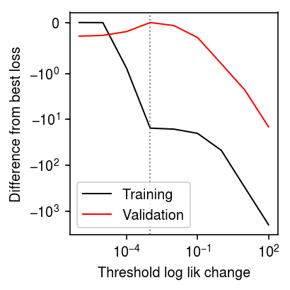
Look at overfitting the training data in WNMF.
nmf_res = []
x, *_ = simulate(n=200, p=300, k=3, pve=1, seed=0)
w = np.random.uniform(size=x.shape) < 0.99
for tol in np.logspace(-6, 2, 9):
  # Important: seed the random initialization
  np.random.seed(100)
  l, f, training_loss = scmodes.lra.nmf(x, w=w, rank=3, tol=tol, max_iters=50000)
  val_loss = -np.where(~w, st.poisson(mu=l @ f.T).logpmf(x), 0).sum()
  nmf_res.append([tol, training_loss, val_loss])
nmf_res = pd.DataFrame(nmf_res, columns=['tol', 'training_loss', 'val_loss'])
plt.clf()
plt.gcf().set_size_inches(3, 3)
plt.xscale('log')
plt.yscale('symlog', linthreshy=1)
plt.plot(nmf_res['tol'], nmf_res['training_loss'].min() - nmf_res['training_loss'], lw=1, c='k', label='Training')
plt.plot(nmf_res['tol'], nmf_res['val_loss'].min() - nmf_res['val_loss'], lw=1, c='r', label='Validation')
plt.axvline(x=nmf_res.loc[nmf_res['val_loss'].idxmin(), 'tol'], lw=1, ls=':', c='0.5')
plt.legend()
plt.ylabel('Difference from best loss')
plt.xlabel('Threshold log lik change')
plt.tight_layout()
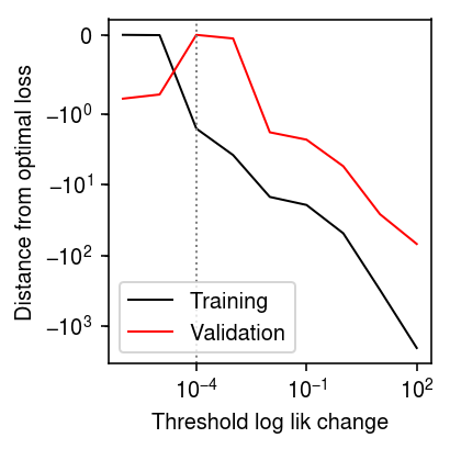
Repeat for 5% missing.
nmf_res = []
x, *_ = simulate(n=200, p=300, k=3, pve=1, seed=0)
w = np.random.uniform(size=x.shape) < 0.95
for tol in np.logspace(-6, 2, 9):
  # Important: seed the random initialization
  np.random.seed(100)
  l, f, training_loss = scmodes.lra.nmf(x, w=w, rank=3, tol=tol, max_iters=50000)
  val_loss = -np.where(~w, st.poisson(mu=l @ f.T).logpmf(x), 0).sum()
  nmf_res.append([tol, training_loss, val_loss])
nmf_res = pd.DataFrame(nmf_res, columns=['tol', 'training_loss', 'val_loss'])
plt.clf()
plt.gcf().set_size_inches(3, 3)
plt.xscale('log')
plt.yscale('symlog', linthreshy=1)
plt.plot(nmf_res['tol'], nmf_res['training_loss'].min() - nmf_res['training_loss'], lw=1, c='k', label='Training')
plt.plot(nmf_res['tol'], nmf_res['val_loss'].min() - nmf_res['val_loss'], lw=1, c='r', label='Validation')
plt.axvline(x=nmf_res.loc[nmf_res['val_loss'].idxmin(), 'tol'], lw=1, ls=':', c='0.5')
plt.legend(loc='lower left')
plt.ylabel('Distance from optimal loss')
plt.xlabel('Threshold log lik change')
plt.tight_layout()
Simulated NB example
Simulate some data from the model.
np.random.seed(0)
n = 500
p = 100
k = 3
l = np.random.lognormal(sigma=.5, size=(n, k))
f = np.random.lognormal(sigma=.5, size=(p, k))
mu = l.dot(f.T)
inv_disp = 0.1
u = np.random.gamma(shape=inv_disp, scale=1 / inv_disp, size=(n, p))
x = np.random.poisson(lam=mu * u)
Zihao Wang previously found that NBMF achieves a worse log likelihood than NMF, even on NB data. Investigate whether this happens in our implementation.
l0, f0, pois_loss = scmodes.lra.nmf(x, rank=3, tol=1e-2, max_iters=10000, verbose=True)
l1, f1, _, nb_loss = scmodes.lra.wnbmf.nbmf(x, rank=3, inv_disp=inv_disp, tol=1e-2, max_iters=10000, fix_inv_disp=True, verbose=True)
l2, f2, inv_disp_hat, nb_loss2 = scmodes.lra.wnbmf.nbmf(x, rank=3, inv_disp=1, tol=1e-2, max_iters=10000, fix_inv_disp=False, verbose=True)
pd.Series({
  'NMF': pois_loss,
  'Oracle': -st.nbinom(n=inv_disp, p=1 / (1 + mu / inv_disp)).logpmf(x).sum(),
  'NMF (oracle phi)': -st.nbinom(n=inv_disp, p=1 / (1 + l0 @ f0.T / inv_disp)).logpmf(x).sum(),
  'NBMF (oracle phi)': nb_loss,
  'NBMF': nb_loss2,
})
NMF                  349729.653625
Oracle                79416.060119
NMF (oracle phi)      78215.149392
NBMF (oracle phi)     78133.257422
NBMF                  78085.164014
dtype: float64
Run the methods.
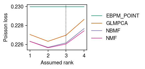
imputation_res = []
for rank in range(1, 5):
  for method in ('oracle', 'ebpm_point', 'wnmf', 'wglmpca', 'wnbmf'):
    print(f'Fitting {method} (rank {rank})')
    loss = getattr(scmodes.benchmark, f'imputation_score_{method}')(
      x,
      rank=rank,
      frac=0.1,
      tol=1e-3,
      max_iters=10000,
      seed=0,
      inv_disp=1,
      fix_inv_disp=False)
    imputation_res.append([method, rank, loss])
imputation_res = pd.DataFrame(imputation_res, columns=['method', 'rank', 'loss'])
Plot the results.
cm = plt.get_cmap('Dark2')
plt.clf()
plt.gcf().set_size_inches(4, 3)
for i, (k, g) in enumerate(imputation_res.groupby('method')):
  plt.plot(g['rank'], g['loss'], lw=1, marker=None, c=cm(i), label=k.upper())
plt.axvline(x=3, lw=1, ls=':', c='k')
plt.legend(frameon=False, loc='center left', bbox_to_anchor=(1, .5))
# plt.xticks(np.arange(1, 11), np.arange(1, 11))
plt.xlabel('Assumed rank')
plt.ylabel('Poisson loss')
plt.tight_layout()
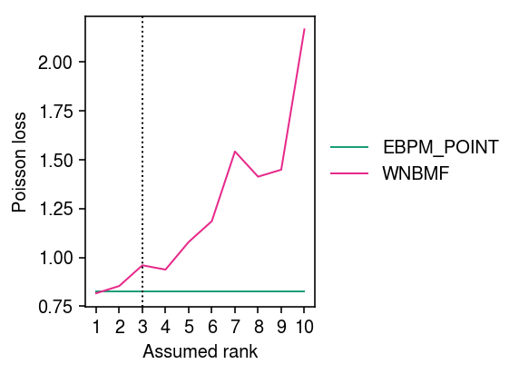
Zoom in on WNBMF and EBPM-Point.
cm = plt.get_cmap('Dark2')
plt.clf()
plt.gcf().set_size_inches(4, 3)
for i, (k, g) in enumerate(imputation_res.groupby('method')):
  if k in ('ebpm_point', 'wnbmf'):
    plt.plot(g['rank'], g['loss'], lw=1, marker=None, c=cm(i), label=k.upper())
plt.axvline(x=3, lw=1, ls=':', c='k')
plt.legend(frameon=False, loc='center left', bbox_to_anchor=(1, .5))
plt.xticks(np.arange(1, 11), np.arange(1, 11))
plt.xlabel('Assumed rank')
plt.ylabel('Poisson loss')
plt.tight_layout()
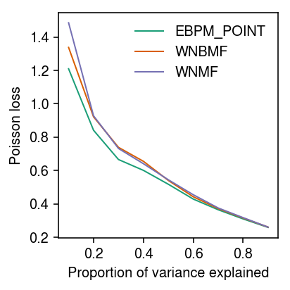
Look at how imputation performance depends on the relative magnitude of the random effect variance \(\phi\) and the structured variance \(\operatorname{Var}(\mu)\). Give each method the oracle rank.
imputation_res = []
for pve in np.linspace(.1, .9, 9):
  for method in ('ebpm_point', 'wnmf', 'wnbmf'):
    x, *_ = simulate(n=500, p=100, k=3, pve=pve, seed=0)
    loss = getattr(scmodes.benchmark, f'imputation_score_{method}')(x, rank=3, frac=0.1, seed=0, inv_disp=1, fix_inv_disp=False)
    imputation_res.append([pve, method, loss])
imputation_res = pd.DataFrame(imputation_res, columns=['pve', 'method', 'loss'])
cm = plt.get_cmap('Dark2')
plt.clf()
plt.gcf().set_size_inches(3, 3)
for i, (k, g) in enumerate(imputation_res.groupby('method')):
  plt.plot(g['pve'], g['loss'], lw=1, c=cm(i), label=k.upper())
plt.legend(frameon=False)
plt.xlabel('Proportion of variance explained')
plt.ylabel('Poisson loss')
plt.tight_layout()
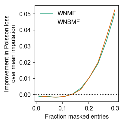
Look at how imputation performance depends on the proportion of masked entries.
imputation_res = []
for frac in np.linspace(.01, .3, 10):
  for method in ('ebpm_point', 'wnmf', 'wnbmf'):
    x, *_ = simulate(n=500, p=100, k=3, pve=0.9, seed=0)
    loss = getattr(scmodes.benchmark, f'imputation_score_{method}')(x, rank=3, frac=frac, seed=0, inv_disp=1, fix_inv_disp=False)
    imputation_res.append([frac, method, loss])
imputation_res = pd.DataFrame(imputation_res, columns=['frac', 'method', 'loss'])
cm = plt.get_cmap('Dark2')
T = imputation_res.pivot(index='frac', columns='method')['loss']
plt.clf()
plt.gcf().set_size_inches(3, 3)
for i, m in enumerate(('wnmf', 'wnbmf')):
  plt.plot(T.index, T['ebpm_point'] - T[m], lw=1, c=cm(i), label=m.upper())
plt.axhline(y=0, lw=1, ls=':', c='k')
plt.legend(frameon=False)
plt.xlabel('Fraction masked entries')
plt.ylabel('Improvement in Poisson loss\nover mean imputation')
plt.tight_layout()
Rank 1 problem
To understand why WNMF/WNBMF do worse than mean imputation when the fraction of masked entries is small, look at a rank 1 problem. First, repeat the analysis varying the fraction of masked entries, fixing the rank of each method to the oracle value.
imputation_res = []
for pve in (0.5, 0.9, 1):
  x, *_ = simulate(n=500, p=100, k=1, pve=pve, seed=0)
  for frac in np.linspace(.01, .3, 10):
    for method in ('ebpm_point', 'wnmf', 'wnbmf'):
      loss = getattr(scmodes.benchmark, f'imputation_score_{method}')(x, rank=1, frac=frac, seed=0, inv_disp=1, fix_inv_disp=False)
      imputation_res.append([pve, frac, method, loss])
imputation_res = pd.DataFrame(imputation_res, columns=['pve', 'frac', 'method', 'loss'])
cm = plt.get_cmap('Paired')
T = imputation_res.pivot_table(index='frac', columns=['method', 'pve'], values='loss')
plt.clf()
plt.gcf().set_size_inches(3.5, 3)
for i, (p, m) in enumerate(it.product((0.5, 0.9, 1), ('wnmf', 'wnbmf'))):
  plt.plot(T.index, T['ebpm_point', p] - T[m, p], lw=1, c=cm(i), label=f'{m.upper()}–{p:.1f}')
plt.axhline(y=0, lw=1, ls=':', c='k')
plt.legend(frameon=False)
plt.xlabel('Fraction masked entries')
plt.ylabel('Improvement in Poisson loss\nover mean imputation')
plt.tight_layout()
![]()
Zoom in around 0 improvement.
cm = plt.get_cmap('Paired')
T = imputation_res.pivot_table(index='frac', columns=['method', 'pve'], values='loss')
plt.clf()
plt.gcf().set_size_inches(3.5, 3)
plt.ylim(-2e-4, 2e-4)
for i, (p, m) in enumerate(it.product((0.5, 0.9, 1), ('wnmf', 'wnbmf'))):
  plt.plot(T.index, T['ebpm_point', p] - T[m, p], lw=1, c=cm(i), label=f'{m.upper()}–{p:.1f}')
plt.axhline(y=0, lw=1, ls=':', c='k')
plt.legend(frameon=False)
plt.xlabel('Fraction masked entries')
plt.ylabel('Improvement in Poisson loss\nover mean imputation')
plt.tight_layout()
![]()
Look at one example where PVE = 0.5.
x, mu, u = simulate(n=500, p=100, k=1, pve=0.5, seed=0)
w = np.random.uniform(size=x.shape) < 0.99

m0 = scmodes.lra.nbmf(x, w=w, rank=1, inv_disp=1, fix_inv_disp=False)
# Fix inverse dispersion to oracle value
m1 = scmodes.lra.nbmf(x, w=w, rank=1, inv_disp=u.var(), fix_inv_disp=True)
# Initialize inverse dispersion to oracle value
m2 = scmodes.lra.nbmf(x, w=w, rank=1, inv_disp=u.var(), fix_inv_disp=False)
Look at the difference in log likelihood between default initialization of inverse dispersion and oracle inverse dispersion.
m0[-1] - m1[-1]
-826.6176850515767
Look at the difference in log likelihood between default initialization and initializing at oracle inverse dispersion.
m0[-1] - m2[-1]
-0.02368231453874614
Look at the difference in imputation performance.
np.array([np.where(w, -st.poisson(mu=m[0] @ m[1].T).logpmf(x), 0).sum() for m in (m0, m1, m2)])
array([72207.27616216, 72227.28379018, 72207.59613526])
Look at mean imputation.
s = (w * x).sum(axis=1)
muhat = (w * x).sum(axis=0) / s.sum()
-np.where(w, st.poisson(mu=np.outer(s, muhat)).logpmf(x), 0).sum()
72185.58560610042
Look at the median absolute difference in the estimated \(\mu_{ij}\) at observed entries.
# Important: in numpy.ma, True = missing
np.ma.median(np.ma.masked_array(abs(x - m0[0] @ m0[1].T), mask=~w))
0.7076492332569424
np.ma.median(np.ma.masked_array(abs(x - np.outer(s, muhat)), mask=~w))
0.7092451591147081
Look at the scatter of predicted \(\mu_{ij}\).
plt.clf()
fig, ax = plt.subplots(2, 2, sharex=True, sharey=True)
fig.set_size_inches(5, 5)

ax[0,0].scatter((m0[0] @ m0[1].T)[w].ravel(), mu[w].ravel(), c='0.7', label='Observed', s=1, alpha=0.1)
ax[0,0].scatter((m0[0] @ m0[1].T)[~w].ravel(), mu[~w].ravel(), c='r', label='Masked', s=1, alpha=0.5)
ax[0,0].set_ylabel('Ground truth $\mu$')
leg = ax[0,0].legend(frameon=False, handletextpad=0, markerscale=4)
for t in leg.legendHandles:
  t.set_alpha(1)

ax[0,1].axis('off')

ax[1,0].scatter((m0[0] @ m0[1].T)[w].ravel(), np.outer(s, muhat)[w].ravel(), c='0.7', label='Observed', s=1, alpha=0.1)
ax[1,0].scatter((m0[0] @ m0[1].T)[~w].ravel(), np.outer(s, muhat)[~w].ravel(), c='r', label='Masked', s=1, alpha=0.5)
ax[1,0].set_xlabel('WNBMF $\hat\mu$')
ax[1,0].set_ylabel('EBPM-Point $\hat\mu$')

ax[1,1].scatter(mu[w].ravel(), np.outer(s, muhat)[w].ravel(), c='0.7', label='Observed', s=1, alpha=0.1)
ax[1,1].scatter(mu[~w].ravel(), np.outer(s, muhat)[~w].ravel(), c='r', label='Masked', s=1, alpha=0.5)
ax[1,1].set_xlabel('Ground truth $\mu$')

fig.tight_layout()
![]()
Look at how imputation performance depends on the scale of \(\mu\). First, look at the typical maximum simulated value.
[simulate(n=500, p=100, k=1, pve=0.5, seed=i)[1].max() for i in range(10)]
[10.52486304374879,
32.94138955233211,
27.056806481363978,
21.39358920123412,
13.6783369842979,
12.004504063906163,
11.943634373434936,
14.671976105187785,
13.467243812000493,
17.786908562734304]
Fix the PVE at 0.5, the fraction of masked entries to 0.05, and the rank to the oracle value. Vary the maximum \(\mu\) by scaling the simulated values.
imputation_res = []
for mu_max in (10, 50, 100):
  x, *_ = simulate(n=500, p=100, k=1, mu_max=mu_max, pve=0.5, seed=0)
  for method in ('ebpm_point', 'wnmf', 'wnbmf'):
    loss = getattr(scmodes.benchmark, f'imputation_score_{method}')(x, rank=1, frac=0.05, seed=0, inv_disp=1, fix_inv_disp=False)
    imputation_res.append([mu_max, method, loss])
imputation_res = pd.DataFrame(imputation_res, columns=['mu_max', 'method', 'loss'])
cm = plt.get_cmap('Dark2')
T = imputation_res.pivot(index='mu_max', columns='method', values='loss')
plt.clf()
plt.gcf().set_size_inches(3, 3)
for i, k in enumerate(['wnmf', 'wnbmf']):
  plt.plot(T.index, T['ebpm_point'] - T[k], lw=1, c=cm(i), label=k.upper())
plt.axhline(y=0, ls=':', lw=1, c='k')
plt.legend(frameon=False)
plt.xlabel('Maximum $\mu$')
plt.ylabel('Improvement in Poisson loss\nover mean imputation')
plt.tight_layout()
![]()
Look at one example.
x, mu, u = simulate(n=500, p=100, k=1, mu_max=100, pve=0.5, seed=0)
w = np.random.uniform(size=x.shape) < 0.99

m0 = scmodes.lra.nbmf(x, w=w, rank=1, inv_disp=1, fix_inv_disp=False, verbose=True)

s = (w * x).sum(axis=1)
muhat = (w * x).sum(axis=0) / s.sum()
plt.clf()
fig, ax = plt.subplots(2, 2, sharex=True, sharey=True)
fig.set_size_inches(5, 5)

ax[0,0].scatter((m0[0] @ m0[1].T)[w].ravel(), mu[w].ravel(), c='0.7', label='Observed', s=1, alpha=0.1)
ax[0,0].scatter((m0[0] @ m0[1].T)[~w].ravel(), mu[~w].ravel(), c='r', label='Masked', s=1, alpha=0.5)
ax[0,0].set_ylabel('Ground truth $\mu$')
leg = ax[0,0].legend(frameon=False, handletextpad=0, markerscale=4)
for t in leg.legendHandles:
  t.set_alpha(1)

ax[0,1].axis('off')

ax[1,0].scatter((m0[0] @ m0[1].T)[w].ravel(), np.outer(s, muhat)[w].ravel(), c='0.7', label='Observed', s=1, alpha=0.1)
ax[1,0].scatter((m0[0] @ m0[1].T)[~w].ravel(), np.outer(s, muhat)[~w].ravel(), c='r', label='Masked', s=1, alpha=0.5)
ax[1,0].set_xlabel('WNBMF $\hat\mu$')
ax[1,0].set_ylabel('EBPM-Point $\hat\mu$')

ax[1,1].scatter(mu[w].ravel(), np.outer(s, muhat)[w].ravel(), c='0.7', label='Observed', s=1, alpha=0.1)
ax[1,1].scatter(mu[~w].ravel(), np.outer(s, muhat)[~w].ravel(), c='r', label='Masked', s=1, alpha=0.5)
ax[1,1].set_xlabel('Ground truth $\mu$')

fig.tight_layout()
![]()