Transformations of deconvolved gene expression distributions
Table of Contents
Introduction
From the perspective of distribution deconvolution, scRNA-seq count data has a mean-variance relationship simply by convolution with a Poisson technical noise model.
Here, we investigate whether the latent gene expression distribution also has a mean-variance relationship, and what happens to it when we transform the distribution.
Setup
import numpy as np
import pandas as pd
import scmodes
%matplotlib inline
%config InlineBackend.figure_formats = set(['retina'])
import matplotlib.pyplot as plt
plt.rcParams['figure.facecolor'] = 'w'
Methods
The key idea of our approach is to deconvolve the gene expression of iPSCs assuming:
\[ x_{ijk} \sim \mathrm{Poisson}(s_{ij} \exp(\mathbf{z}_i' \mathbf{b}_j) \lambda_{ijk}) \]
\[ \lambda_{ijk} \sim g_{ik}(\cdot) = \pi_{ik} \delta_0(\cdot) + (1 - \pi_{ik}) \mathrm{Gamma}(\mu_{ik}, \phi_{ik}) \]
From the fitted \(\hat{g}_1, \ldots, \hat{g}_p\), we can investigate whether there is a mean-variance relationship in latent gene expression.
Results
Untransformed distribution
Read the deconvolved distributions.
log_mu = pd.read_csv('/project2/mstephens/aksarkar/projects/singlecell-qtl/data/density-estimation/design1/zi2-log-mu.txt.gz', sep=' ', index_col=0)
log_phi = pd.read_csv('/project2/mstephens/aksarkar/projects/singlecell-qtl/data/density-estimation/design1/zi2-log-phi.txt.gz', sep=' ', index_col=0)
logodds = pd.read_csv('/project2/mstephens/aksarkar/projects/singlecell-qtl/data/density-estimation/design1/zi2-logodds.txt.gz', sep=' ', index_col=0)
Throw out the individual with evidence of contamination.
for x in (log_mu, log_phi, logodds):
  del x['NA18498']
Recover the mean and variance of latent gene expression per gene, per individual.
# Important: log(sigmoid(x)) = -softplus(-x)
mean = np.exp(log_mu - np.log1p(np.exp(logodds)))
variance = np.exp(2 * log_mu + log_phi - np.log1p(np.exp(logodds))) + np.exp(-np.log1p(np.exp(logodds)) - np.log1p(np.exp(-logodds)) + 2 * log_mu)
Plot the mean/variance relationship.
plt.clf()
plt.gcf().set_size_inches(3, 3)
plt.semilogx()
plt.semilogy()
plt.scatter(mean.values.ravel(), variance.values.ravel(), c='k', s=4, alpha=0.1)
plt.xlabel('Latent gene expression mean')
plt.ylabel('Latent gene expression variance')
Text(0, 0.5, 'Latent gene expression variance')

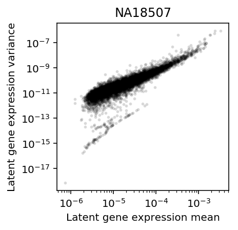
Restrict to the individual with the most cells (\(n=284\)).
plt.clf()
plt.gcf().set_size_inches(3, 3)
plt.semilogx()
plt.semilogy()
plt.scatter(mean['NA18507'], variance['NA18507'].values.ravel(), c='k', s=4, alpha=0.1)
plt.title('NA18507')
plt.xlabel('Latent gene expression mean')
plt.ylabel('Latent gene expression variance')
Text(0, 0.5, 'Latent gene expression variance')
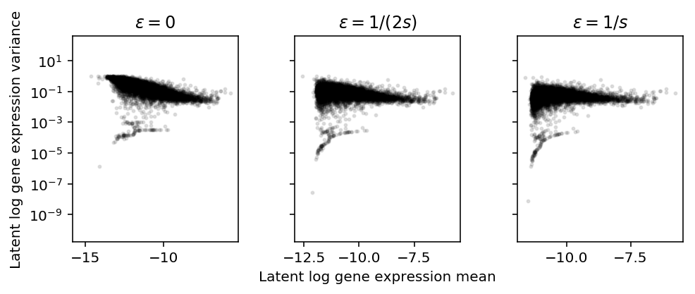
Log transform
Assume \(\lambda_{ijk} \sim g_{ik}(\cdot)\), as above. Plot the approximate relationship between \(E[\ln(\lambda + \epsilon)]\) and \(V[\ln(\lambda + \epsilon)]\) by first-order Taylor expansion.
\[ E[\ln(x + \epsilon)] \approx \ln(E[x] + \epsilon) - \frac{V[x]}{2 (E[x] + \epsilon)^2} \]
\[ V[\ln(x + \epsilon)] \approx \frac{V[x]}{(E[x] + \epsilon)^2} - \frac{V[x]^2}{4 (E[x] + \epsilon)^4} \]
Importantly, \(\epsilon\) needs to be on the same scale as \(\lambda\). But \(x_{ijk} \sim \mathrm{Poisson}(s_{ij} \lambda_{ijk})\), so \(\lambda_{ijk}\) is on the scale of \(1 / s_{ij}\). Instead of assuming \(x_{ijk} \sim F_{ijk}(\cdot)\), assume:
\[ x_{ijk} \sim \frac{1}{n} \sum_j F_{ijk}(\cdot) \]
Then, \(E[x_{ijk}] = \frac{1}{n}\sum_j s_{ij} E[\lambda_{ijk}]\). This gives us a single scaling factor for \(g_{ik}\).
Read the metadata for the iPSCs.
annotations = pd.read_csv('/project2/mstephens/aksarkar/projects/singlecell-qtl/data/scqtl-annotation.txt', sep='\t')
keep_samples = pd.read_csv('/project2/mstephens/aksarkar/projects/singlecell-qtl/data/quality-single-cells.txt', sep='\t', index_col=0, header=None)
annotations = annotations.loc[keep_samples.values.ravel()]
s = annotations.loc[(annotations['chip_id'] == 'NA18507').values, 'mol_hs'].mean()
plt.clf()
fig, ax = plt.subplots(1, 3, sharey=True)
fig.set_size_inches(7, 3)
for a, eps, t in zip(ax, np.array([0, 0.5, 1]) / s, ['0', '1/(2s)', '1/s']):
  a.set_yscale('log')
  m = np.log(mean['NA18507'] + eps) - variance['NA18507'] / (2 * np.square(mean['NA18507'] + eps))
  v = variance['NA18507'] / np.square(mean['NA18507'] + eps) - np.square(variance['NA18507']) / (4 * (mean['NA18507'] + eps) ** 4)
  a.scatter(m, v, c='k', s=4, alpha=0.1)
  a.set_title(f'$\epsilon = {t}$')
ax[1].set_xlabel('Latent log gene expression mean')
ax[0].set_ylabel('Latent log gene expression variance')
fig.tight_layout()
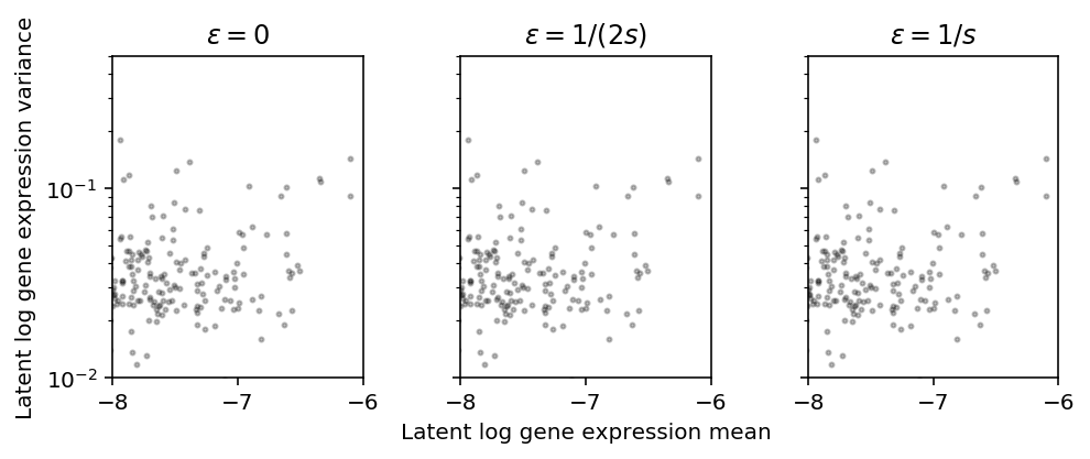
Zoom in on highly expressed genes.
plt.clf()
fig, ax = plt.subplots(1, 3, sharey=True)
fig.set_size_inches(7, 3)
for a, eps, t in zip(ax, np.array([0, 0.5, 1]) / s, ['0', '1/(2s)', '1/s']):
  a.set_yscale('log')
  a.set_xlim(-8, -6)
  a.set_ylim(1e-2, .5)
  a.scatter(m, v, c='k', s=4, alpha=0.25)
  a.set_title(f'$\epsilon = {t}$')
ax[1].set_xlabel('Latent log gene expression mean')
ax[0].set_ylabel('Latent log gene expression variance')
fig.tight_layout()
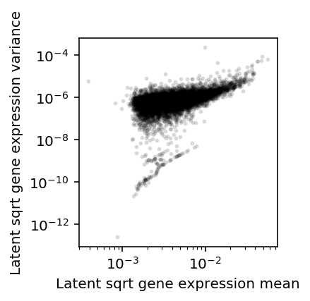
Square root transform
Assume \(\lambda_{ijk} \sim g_{ik}(\cdot)\), as above. Plot the approximate relationship between \(E[\lambda^{1/2}]\) and \(V[\lambda^{1/2}]\) by first-order Taylor expansion.
\[ E[x^{1/2}] \approx (E[x])^{1/2} - \frac{V[x]}{8 E[x]^{3/2}} \]
\[ V[x^{1/2}] \approx \frac{V[x]}{4 E[x]} - \frac{V[x]^2}{64 E[x]^3} \]
plt.clf()
plt.gcf().set_size_inches(3, 3)
plt.semilogx()
plt.semilogy()
m = np.sqrt(mean['NA18507']) - variance['NA18507'] / (8 * np.power(mean['NA18507'], 1.5))
v = variance['NA18507'] / (4 * mean['NA18507']) - np.square(variance['NA18507']) / (64 * np.power(mean['NA18507'], 3))
plt.scatter(m, v, c='k', s=4, alpha=0.1)
plt.xlabel('Latent sqrt gene expression mean')
plt.ylabel('Latent sqrt gene expression variance')
plt.gcf().tight_layout()
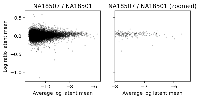
Variance effects versus mean effects
After convolution of a Gamma with a Poisson, we expect a quadratic mean-variance relationship. But we showed above that after deconvolution, we still see a linear mean-variance relationship within samples.
What if we look between conditions? To investigate this, look at MA plots of latent gene expression for two different donor individuals.
Find the individual with the second-most cells.
annotations['chip_id'].value_counts().sort_values(ascending=False).head(n=2)
NA18507    284
NA18501    221
Name: chip_id, dtype: int64
a = np.log(mean['NA18507'] + 1 / annotations.loc[(annotations['chip_id'] == 'NA18507').values, 'mol_hs'].mean())
b = np.log(mean['NA18501'] + 1 / annotations.loc[(annotations['chip_id'] == 'NA18501').values, 'mol_hs'].mean())
plt.clf()
fig, ax = plt.subplots(1, 2, sharey=True)
fig.set_size_inches(6, 3)
ax[0].scatter((a + b) / 2, a - b, s=2, c='k', alpha=0.2)
ax[0].axhline(y=0, ls=':', lw=1, c='r')
ax[0].set_title('NA18507 / NA18501')
ax[1].scatter((a + b) / 2, a - b, s=2, c='k', alpha=0.2)
ax[1].axhline(y=0, ls=':', lw=1, c='r')
ax[1].set_xlim(-8, ax[0].get_xlim()[1])
ax[1].set_title('NA18507 / NA18501 (zoomed)')
for a in ax:
  a.set_xlabel('Average log latent mean')
ax[0].set_ylabel('Log ratio latent mean')
fig.tight_layout()
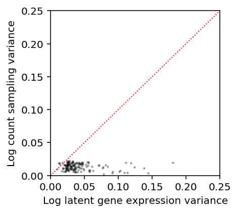
Comparison of sampling variance with biological variance
From the perspective of deconvolution, biological variance describes \(\lambda \sim g(\cdot)\), while sampling variance describes \(x \mid s, \lambda \sim \mathrm{Poisson}(s \lambda)\).
Our results above suggest that for the highest expressed genes, \(V[\ln(\lambda + 1 / s)]\) is order \(10^{-1}\). Estimate the sampling variance \(V[\ln(x + 1) \mid s, \lambda=\mu]\) for genes with \(E[\ln(\lambda + 1 / s)] > -8\), where \(\mu = E[\lambda]\).
s = annotations.loc[(annotations['chip_id'] == 'NA18507').values, 'mol_hs'].mean()
m = np.log(mean['NA18507'] + 1 / s) - variance['NA18507'] / (2 * np.square(mean['NA18507'] + 1 / s))
v = variance['NA18507'] / np.square(mean['NA18507'] + 1 / s) - np.square(variance['NA18507']) / (4 * (mean['NA18507'] + 1 / s) ** 4)
query = m[m > -8].index
ipsc = scmodes.dataset.ipsc('/project2/mstephens/aksarkar/projects/singlecell-qtl/data/', query=query, return_df=True)
subset = ipsc[(annotations['chip_id'] == 'NA18507').values.ravel()]
lam = s * mean['NA18507']
vx = lam / np.square(lam + 1) - np.square(lam) / (4 * (lam + 1) ** 4)
plt.clf()
plt.gcf().set_size_inches(3, 3)
plt.scatter(v[m > -8], vx[m > -8], c='k', s=2, alpha=0.25)
plt.plot([0, .25], [0, .25], ls=':', lw=1, c='r')
plt.xlim([0, .25])
plt.ylim([0, .25])
plt.xlabel('Log latent gene expression variance')
_ = plt.ylabel('Log count sampling variance')