Randomized quantiles
Table of Contents
Introduction
We previously illustrated an example of our approach to testing GOF using real data. Here, we characterize the variability in the randomized quantiles that went into that illustration.
Setup
import anndata
import numpy as np
import pandas as pd
import scipy.optimize as so
import scipy.special as sp
import scipy.stats as st
import scmodes
import sqlite3
import rpy2.robjects.packages
import rpy2.robjects.pandas2ri
rpy2.robjects.pandas2ri.activate()
ashr = rpy2.robjects.packages.importr('ashr')
%matplotlib inline
%config InlineBackend.figure_formats = set(['retina'])
import colorcet
import matplotlib.pyplot as plt
plt.rcParams['figure.facecolor'] = 'w'
plt.rcParams['font.family'] = 'Nimbus Sans'
Data
Read the data.
gene_info = pd.read_csv('/project2/mstephens/aksarkar/projects/singlecell-qtl/data/scqtl-genes.txt.gz', sep='\t', index_col=0)
cytotoxic_t = scmodes.dataset.read_10x('/project2/mstephens/aksarkar/projects/singlecell-ideas/data/10xgenomics/cytotoxic_t/filtered_matrices_mex/hg19/', return_df=True)
gene = 'ENSG00000109475'
x = cytotoxic_t.loc[:,gene]
s = cytotoxic_t.sum(axis=1)
y = np.arange(x.max() + 1)
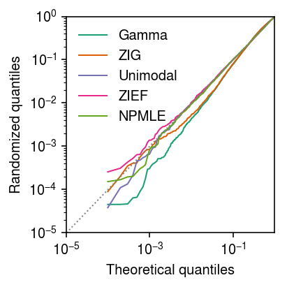
Seed 2
Generate an independent draw of randomized quantiles.
rpp = dict()
pmf = dict()
np.random.seed(2)
gamma_res = scmodes.ebpm.ebpm_gamma(x, s)
rpp['Gamma'] = scmodes.benchmark.gof._rpp(
  scmodes.benchmark.gof._zig_cdf(x - 1, size=s, log_mu=gamma_res[0], log_phi=-gamma_res[1]),
  scmodes.benchmark.gof._zig_pmf(x, size=s, log_mu=gamma_res[0], log_phi=-gamma_res[1]))
pmf['Gamma'] = np.array([scmodes.benchmark.gof._zig_pmf(k, size=s, log_mu=gamma_res[0], log_phi=-gamma_res[1]).mean()
                         for k in y])

point_gamma_res = scmodes.ebpm.ebpm_point_gamma(x, s)
rpp['ZIG'] = scmodes.benchmark.gof._rpp(
  scmodes.benchmark.gof._zig_cdf(x - 1, size=s, log_mu=point_gamma_res[0], log_phi=-point_gamma_res[1], logodds=point_gamma_res[2]),
  scmodes.benchmark.gof._zig_pmf(x, size=s, log_mu=point_gamma_res[0], log_phi=-point_gamma_res[1], logodds=point_gamma_res[2]))
pmf['ZIG'] = np.array([scmodes.benchmark.gof._zig_pmf(k, size=s, log_mu=point_gamma_res[0], log_phi=-point_gamma_res[1], logodds=point_gamma_res[2]).mean()
                       for k in y])

zief_res = scmodes.ebpm.ebpm_point_expfam(x, s)
rpp['ZIEF'] = scmodes.benchmark.gof._rpp(
  scmodes.benchmark.gof._point_expfam_cdf(x.values.ravel() - 1, size=s, res=zief_res),
  scmodes.benchmark.gof._point_expfam_pmf(x.values.ravel(), size=s, res=zief_res))
# We need np.full here because _point_expfam_pmf does not broadcast
pmf['ZIEF'] = np.array([scmodes.benchmark.gof._point_expfam_pmf(np.full(x.shape, k), size=s, res=zief_res).mean()
                        for k in y])

unimodal_res = scmodes.ebpm.ebpm_unimodal(x, s)
rpp['Unimodal'] = scmodes.benchmark.gof._rpp(
  scmodes.benchmark.gof._ash_cdf(x - 1, s=s, fit=unimodal_res),
  scmodes.benchmark.gof._ash_pmf(x, s=s, fit=unimodal_res))
# It is simpler to compute this here than to mess with the ash_data object
g = np.array(unimodal_res.rx2('fitted_g'))
a = np.fmin(g[1], g[2])
b = np.fmax(g[1], g[2])
comp_dens_conv = np.array([((st.gamma(a=k + 1, scale=1 / s.values.reshape(-1, 1)).cdf(b.reshape(1, -1)) - st.gamma(a=k + 1, scale=1 / s.values.reshape(-1, 1)).cdf(a.reshape(1, -1))) / np.outer(s, b - a)).mean(axis=0) for k in y])
comp_dens_conv[:,0] = st.poisson(mu=s.values.reshape(-1, 1) * b[0]).pmf(y).mean(axis=0)
pmf['Unimodal'] = comp_dens_conv @ g[0]

npmle_res = scmodes.ebpm.ebpm_npmle(x, s)
rpp['NPMLE'] = scmodes.benchmark.gof._rpp(
  scmodes.benchmark.gof._ash_cdf(x - 1, s=s, fit=npmle_res),
  scmodes.benchmark.gof._ash_pmf(x, s=s, fit=npmle_res))
g = np.array(npmle_res.rx2('fitted_g'))
a = np.fmin(g[1], g[2])
b = np.fmax(g[1], g[2])
comp_dens_conv = np.array([((st.gamma(a=k + 1, scale=1 / s.values.reshape(-1, 1)).cdf(b.reshape(1, -1)) - st.gamma(a=k + 1, scale=1 / s.values.reshape(-1, 1)).cdf(a.reshape(1, -1))) / np.outer(s, b - a)).mean(axis=0) for k in y])
pmf['NPMLE'] = comp_dens_conv @ g[0]
Plot the randomized quantiles against uniform quantiles.
plt.clf()
plt.gcf().set_size_inches(3, 3)
grid = np.linspace(0, 1, x.shape[0] + 1)[1:]
plt.xscale('log')
plt.yscale('log')
for c, k in zip(plt.get_cmap('Dark2').colors, ['Gamma', 'ZIG', 'Unimodal', 'ZIEF', 'NPMLE']):
  if k in rpp:
    plt.plot(grid, np.sort(rpp[k]), color=c, lw=1, marker=None, label=k)
plt.plot([1e-5, 1], [1e-5, 1], lw=1, ls=':', c='0.5')
plt.legend(frameon=False)
plt.xlim(1e-5, 1)
plt.ylim(1e-5, 1)
plt.xlabel('Theoretical quantiles')
plt.ylabel('Randomized quantiles')
plt.tight_layout()
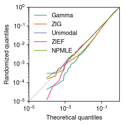
Seed 3
Generate an independent draw of randomized quantiles.
rpp = dict()
pmf = dict()
np.random.seed(3)
gamma_res = scmodes.ebpm.ebpm_gamma(x, s)
rpp['Gamma'] = scmodes.benchmark.gof._rpp(
  scmodes.benchmark.gof._zig_cdf(x - 1, size=s, log_mu=gamma_res[0], log_phi=-gamma_res[1]),
  scmodes.benchmark.gof._zig_pmf(x, size=s, log_mu=gamma_res[0], log_phi=-gamma_res[1]))
pmf['Gamma'] = np.array([scmodes.benchmark.gof._zig_pmf(k, size=s, log_mu=gamma_res[0], log_phi=-gamma_res[1]).mean()
                         for k in y])

point_gamma_res = scmodes.ebpm.ebpm_point_gamma(x, s)
rpp['ZIG'] = scmodes.benchmark.gof._rpp(
  scmodes.benchmark.gof._zig_cdf(x - 1, size=s, log_mu=point_gamma_res[0], log_phi=-point_gamma_res[1], logodds=point_gamma_res[2]),
  scmodes.benchmark.gof._zig_pmf(x, size=s, log_mu=point_gamma_res[0], log_phi=-point_gamma_res[1], logodds=point_gamma_res[2]))
pmf['ZIG'] = np.array([scmodes.benchmark.gof._zig_pmf(k, size=s, log_mu=point_gamma_res[0], log_phi=-point_gamma_res[1], logodds=point_gamma_res[2]).mean()
                       for k in y])

zief_res = scmodes.ebpm.ebpm_point_expfam(x, s)
rpp['ZIEF'] = scmodes.benchmark.gof._rpp(
  scmodes.benchmark.gof._point_expfam_cdf(x.values.ravel() - 1, size=s, res=zief_res),
  scmodes.benchmark.gof._point_expfam_pmf(x.values.ravel(), size=s, res=zief_res))
# We need np.full here because _point_expfam_pmf does not broadcast
pmf['ZIEF'] = np.array([scmodes.benchmark.gof._point_expfam_pmf(np.full(x.shape, k), size=s, res=zief_res).mean()
                        for k in y])

unimodal_res = scmodes.ebpm.ebpm_unimodal(x, s)
rpp['Unimodal'] = scmodes.benchmark.gof._rpp(
  scmodes.benchmark.gof._ash_cdf(x - 1, s=s, fit=unimodal_res),
  scmodes.benchmark.gof._ash_pmf(x, s=s, fit=unimodal_res))
# It is simpler to compute this here than to mess with the ash_data object
g = np.array(unimodal_res.rx2('fitted_g'))
a = np.fmin(g[1], g[2])
b = np.fmax(g[1], g[2])
comp_dens_conv = np.array([((st.gamma(a=k + 1, scale=1 / s.values.reshape(-1, 1)).cdf(b.reshape(1, -1)) - st.gamma(a=k + 1, scale=1 / s.values.reshape(-1, 1)).cdf(a.reshape(1, -1))) / np.outer(s, b - a)).mean(axis=0) for k in y])
comp_dens_conv[:,0] = st.poisson(mu=s.values.reshape(-1, 1) * b[0]).pmf(y).mean(axis=0)
pmf['Unimodal'] = comp_dens_conv @ g[0]

npmle_res = scmodes.ebpm.ebpm_npmle(x, s)
rpp['NPMLE'] = scmodes.benchmark.gof._rpp(
  scmodes.benchmark.gof._ash_cdf(x - 1, s=s, fit=npmle_res),
  scmodes.benchmark.gof._ash_pmf(x, s=s, fit=npmle_res))
g = np.array(npmle_res.rx2('fitted_g'))
a = np.fmin(g[1], g[2])
b = np.fmax(g[1], g[2])
comp_dens_conv = np.array([((st.gamma(a=k + 1, scale=1 / s.values.reshape(-1, 1)).cdf(b.reshape(1, -1)) - st.gamma(a=k + 1, scale=1 / s.values.reshape(-1, 1)).cdf(a.reshape(1, -1))) / np.outer(s, b - a)).mean(axis=0) for k in y])
pmf['NPMLE'] = comp_dens_conv @ g[0]
Plot the randomized quantiles against uniform quantiles.
plt.clf()
plt.gcf().set_size_inches(3, 3)
grid = np.linspace(0, 1, x.shape[0] + 1)[1:]
plt.xscale('log')
plt.yscale('log')
for c, k in zip(plt.get_cmap('Dark2').colors, ['Gamma', 'ZIG', 'Unimodal', 'ZIEF', 'NPMLE']):
  if k in rpp:
    plt.plot(grid, np.sort(rpp[k]), color=c, lw=1, marker=None, label=k)
plt.plot([1e-5, 1], [1e-5, 1], lw=1, ls=':', c='0.5')
plt.legend(frameon=False)
plt.xlim(1e-5, 1)
plt.ylim(1e-5, 1)
plt.xlabel('Theoretical quantiles')
plt.ylabel('Randomized quantiles')
plt.tight_layout()
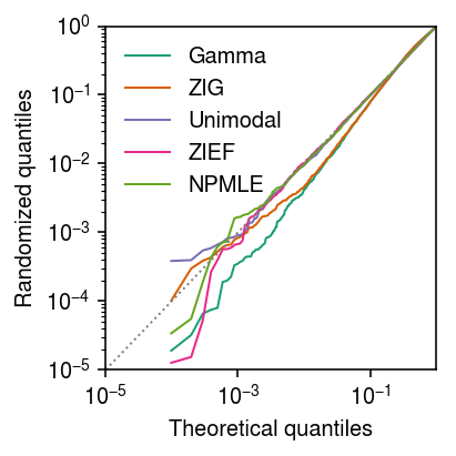
Seed 10
Generate an independent draw of randomized quantiles.
rpp = dict()
pmf = dict()
np.random.seed(10)
gamma_res = scmodes.ebpm.ebpm_gamma(x, s)
rpp['Gamma'] = scmodes.benchmark.gof._rpp(
  scmodes.benchmark.gof._zig_cdf(x - 1, size=s, log_mu=gamma_res[0], log_phi=-gamma_res[1]),
  scmodes.benchmark.gof._zig_pmf(x, size=s, log_mu=gamma_res[0], log_phi=-gamma_res[1]))
pmf['Gamma'] = np.array([scmodes.benchmark.gof._zig_pmf(k, size=s, log_mu=gamma_res[0], log_phi=-gamma_res[1]).mean()
                         for k in y])

point_gamma_res = scmodes.ebpm.ebpm_point_gamma(x, s)
rpp['ZIG'] = scmodes.benchmark.gof._rpp(
  scmodes.benchmark.gof._zig_cdf(x - 1, size=s, log_mu=point_gamma_res[0], log_phi=-point_gamma_res[1], logodds=point_gamma_res[2]),
  scmodes.benchmark.gof._zig_pmf(x, size=s, log_mu=point_gamma_res[0], log_phi=-point_gamma_res[1], logodds=point_gamma_res[2]))
pmf['ZIG'] = np.array([scmodes.benchmark.gof._zig_pmf(k, size=s, log_mu=point_gamma_res[0], log_phi=-point_gamma_res[1], logodds=point_gamma_res[2]).mean()
                       for k in y])

zief_res = scmodes.ebpm.ebpm_point_expfam(x, s)
rpp['ZIEF'] = scmodes.benchmark.gof._rpp(
  scmodes.benchmark.gof._point_expfam_cdf(x.values.ravel() - 1, size=s, res=zief_res),
  scmodes.benchmark.gof._point_expfam_pmf(x.values.ravel(), size=s, res=zief_res))
# We need np.full here because _point_expfam_pmf does not broadcast
pmf['ZIEF'] = np.array([scmodes.benchmark.gof._point_expfam_pmf(np.full(x.shape, k), size=s, res=zief_res).mean()
                        for k in y])

unimodal_res = scmodes.ebpm.ebpm_unimodal(x, s)
rpp['Unimodal'] = scmodes.benchmark.gof._rpp(
  scmodes.benchmark.gof._ash_cdf(x - 1, s=s, fit=unimodal_res),
  scmodes.benchmark.gof._ash_pmf(x, s=s, fit=unimodal_res))
# It is simpler to compute this here than to mess with the ash_data object
g = np.array(unimodal_res.rx2('fitted_g'))
a = np.fmin(g[1], g[2])
b = np.fmax(g[1], g[2])
comp_dens_conv = np.array([((st.gamma(a=k + 1, scale=1 / s.values.reshape(-1, 1)).cdf(b.reshape(1, -1)) - st.gamma(a=k + 1, scale=1 / s.values.reshape(-1, 1)).cdf(a.reshape(1, -1))) / np.outer(s, b - a)).mean(axis=0) for k in y])
comp_dens_conv[:,0] = st.poisson(mu=s.values.reshape(-1, 1) * b[0]).pmf(y).mean(axis=0)
pmf['Unimodal'] = comp_dens_conv @ g[0]

npmle_res = scmodes.ebpm.ebpm_npmle(x, s)
rpp['NPMLE'] = scmodes.benchmark.gof._rpp(
  scmodes.benchmark.gof._ash_cdf(x - 1, s=s, fit=npmle_res),
  scmodes.benchmark.gof._ash_pmf(x, s=s, fit=npmle_res))
g = np.array(npmle_res.rx2('fitted_g'))
a = np.fmin(g[1], g[2])
b = np.fmax(g[1], g[2])
comp_dens_conv = np.array([((st.gamma(a=k + 1, scale=1 / s.values.reshape(-1, 1)).cdf(b.reshape(1, -1)) - st.gamma(a=k + 1, scale=1 / s.values.reshape(-1, 1)).cdf(a.reshape(1, -1))) / np.outer(s, b - a)).mean(axis=0) for k in y])
pmf['NPMLE'] = comp_dens_conv @ g[0]
Plot the randomized quantiles against uniform quantiles.
plt.clf()
plt.gcf().set_size_inches(3, 3)
grid = np.linspace(0, 1, x.shape[0] + 1)[1:]
plt.xscale('log')
plt.yscale('log')
for c, k in zip(plt.get_cmap('Dark2').colors, ['Gamma', 'ZIG', 'Unimodal', 'ZIEF', 'NPMLE']):
  if k in rpp:
    plt.plot(grid, np.sort(rpp[k]), color=c, lw=1, marker=None, label=k)
plt.plot([1e-5, 1], [1e-5, 1], lw=1, ls=':', c='0.5')
plt.legend(frameon=False)
plt.xlim(1e-5, 1)
plt.ylim(1e-5, 1)
plt.xlabel('Theoretical quantiles')
plt.ylabel('Randomized quantiles')
plt.tight_layout()
Expected randomized quantiles
The randomized quantiles are
\begin{equation} u_i \mid x_i \sim \operatorname{Uniform}(\hat{F}(x - 1), \hat{F}(x)) \end{equation}for \(i = 1, \ldots, n\); therefore, their expected value is
\begin{equation} \operatorname{E}[u_i \mid x_i] = \frac{\hat{F}(x - 1) + \hat{F}(x)}{2} = \hat{F}(x - 1) + \frac{1}{2}\hat{f}(x). \end{equation}Assuming \(x \sim \hat{F}\), \(u_i \sim \operatorname{Uniform}(0, 1)\) and the \(k\)th order statistic
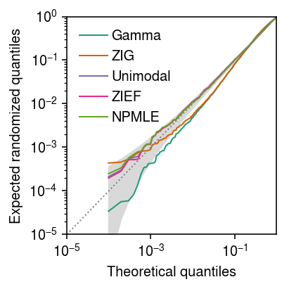
\begin{equation} u_{(k)} \sim \operatorname{Beta}(k, n - k + 1). \end{equation}Plot the expected randomized quantiles against Uniform quantiles. Superimpose the \((0.025, 0.975)\) quantiles of the distribution of Uniform order statistics.
erpp = dict()
gamma_res = scmodes.ebpm.ebpm_gamma(x, s)
erpp['Gamma'] = (scmodes.benchmark.gof._zig_cdf(x - 1, size=s, log_mu=gamma_res[0], log_phi=-gamma_res[1]) +
                 .5 * scmodes.benchmark.gof._zig_pmf(x, size=s, log_mu=gamma_res[0], log_phi=-gamma_res[1]))

point_gamma_res = scmodes.ebpm.ebpm_point_gamma(x, s)
erpp['ZIG'] = (scmodes.benchmark.gof._zig_cdf(x - 1, size=s, log_mu=point_gamma_res[0], log_phi=-point_gamma_res[1], logodds=-point_gamma_res[2]) +
               .5 * scmodes.benchmark.gof._zig_pmf(x, size=s, log_mu=point_gamma_res[0], log_phi=-point_gamma_res[1], logodds=-point_gamma_res[2]))

zief_res = scmodes.ebpm.ebpm_point_expfam(x, s)
erpp['ZIEF'] = (scmodes.benchmark.gof._point_expfam_cdf(x.values.ravel() - 1, size=s, res=zief_res) +
                .5 * scmodes.benchmark.gof._point_expfam_pmf(x.values.ravel(), size=s, res=zief_res))

unimodal_res = scmodes.ebpm.ebpm_unimodal(x, s)
erpp['Unimodal'] = (scmodes.benchmark.gof._ash_cdf(x - 1, s=s, fit=unimodal_res) +
                    .5 * scmodes.benchmark.gof._ash_pmf(x, s=s, fit=unimodal_res))

npmle_res = scmodes.ebpm.ebpm_npmle(x, s)
erpp['NPMLE'] = (scmodes.benchmark.gof._ash_cdf(x - 1, s=s, fit=npmle_res) +
                 .5 * scmodes.benchmark.gof._ash_pmf(x, s=s, fit=npmle_res))
grid = np.linspace(0, 1, x.shape[0] + 1)[1:]
F = st.beta(np.arange(1, 1 + x.shape[0]), 1 + x.shape[0] - np.arange(1, 1 + x.shape[0]))

plt.clf()
plt.gcf().set_size_inches(3, 3)
plt.xscale('log')
plt.yscale('log')
for c, k in zip(plt.get_cmap('Dark2').colors, ['Gamma', 'ZIG', 'Unimodal', 'ZIEF', 'NPMLE']):
  if k in erpp:
    plt.plot(grid, np.sort(erpp[k]), color=c, lw=1, marker=None, label=k)
plt.fill_between(grid, F.ppf(.025), F.ppf(.975), color='0.85')
plt.legend(frameon=False, handletextpad=0.25)
lim = [1e-5, 1]
plt.plot(lim, lim, lw=1, ls=':', c='0.5')
plt.xlim(lim)
plt.ylim(lim)
plt.xlabel('Theoretical quantiles')
plt.ylabel('Expected randomized quantiles')
plt.tight_layout()
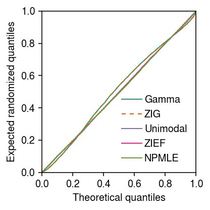
Plot the expected randomized quantiles on a linear scale.
grid = np.linspace(0, 1, x.shape[0] + 1)[1:]
plt.clf()
plt.gcf().set_size_inches(3, 3)
for c, k in zip(plt.get_cmap('Dark2').colors, ['Gamma', 'ZIG', 'Unimodal', 'ZIEF', 'NPMLE']):
  if k == 'ZIG':
    ls = (0, (4, 4))
  else:
    ls = '-'
  if k in erpp:
    plt.plot(grid, np.sort(erpp[k]), color=c, lw=1, ls=ls, marker=None, label=k)
plt.legend(frameon=False, handletextpad=0.25)
lim = [0, 1]
plt.plot(lim, lim, lw=1, ls=':', c='0.5')
plt.xlim(lim)
plt.ylim(lim)
plt.xlabel('Theoretical quantiles')
plt.ylabel('Expected randomized quantiles')
plt.tight_layout()
Gamma model
Look at the estimated Gamma model parameters.
pd.Series({k: v for k, v in zip(('log_mean', 'log_inv_disp', 'llik'), gamma_res)})
log_mean           -4.567842
log_inv_disp        2.392556
llik           -31464.243518
dtype: float64
Look at the estimated point-Gamma model parameters.
pd.Series({k: v for k, v in zip(('log_mean', 'log_inv_disp', 'logodds', 'llik'), point_gamma_res)})
log_mean           -4.567096
log_inv_disp        2.404508
logodds            -7.125454
llik           -31459.278213
dtype: float64
Estimate how many excess zeros in this data are predicted by the point-Gamma model.
sp.expit(point_gamma_res[2]) * x.shape[0]
8.205192265041903
Compute the difference in marginal log likelihood between a point-Gamma and a Gamma expression model.
point_gamma_res[-1] - gamma_res[-1]
4.965304532452137
Compute the difference in marginal log likelihood between a unimodal and a Gamma expression model.
np.array(unimodal_res.rx2('loglik')) - gamma_res[-1]
array([265.32446831])
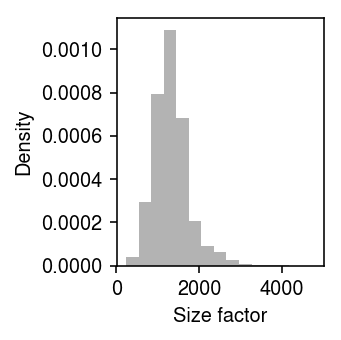
Dependency on size factors
Look at the distribution of size factors.
plt.clf()
plt.gcf().set_size_inches(2.5, 2.5)
plt.hist(s, bins=15, density=True, color='0.7')
plt.xlabel('Size factor')
plt.ylabel('Density')
plt.tight_layout()
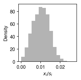
Look at the distribution of \(x_{ij} / x_{i+}\).
plt.clf()
plt.gcf().set_size_inches(2.5, 2.5)
plt.hist(x / s, bins=15, density=True, color='0.7')
plt.xlabel('$x_i / s_i$')
plt.ylabel('Density')
plt.tight_layout()
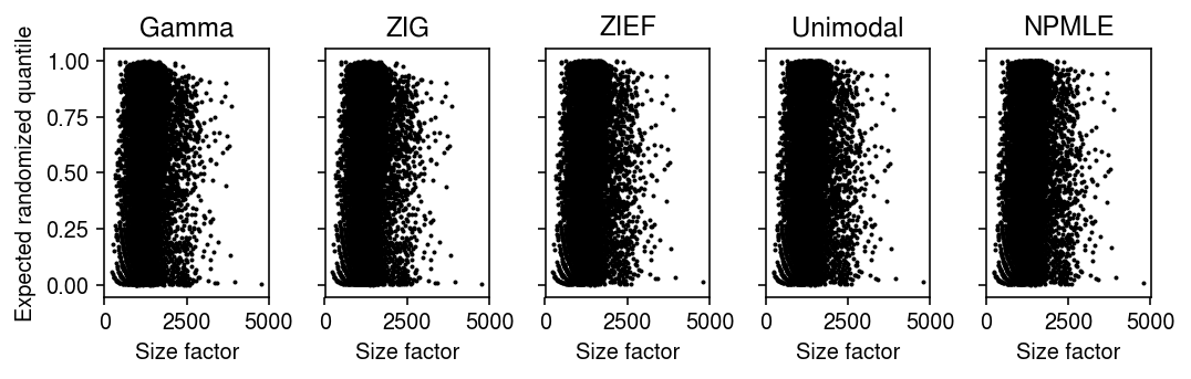
Plot the expected randomized quantile against the size factor, to see if they are not independent.
plt.clf()
fig, ax = plt.subplots(1, 5, sharey=True)
fig.set_size_inches(7.5, 2.5)
for a, k in zip(ax, erpp):
  a.scatter(s, erpp[k], s=1, c='k')
  a.set_title(k)
  a.set_xlabel('Size factor')
ax[0].set_ylabel('Expected randomized quantile')
fig.tight_layout()
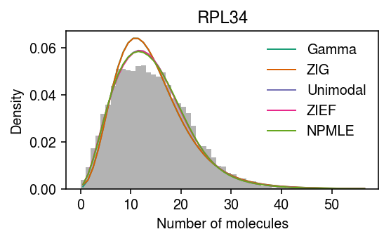
Plot the example again.
pmf = dict()
pmf['Gamma'] = np.array([scmodes.benchmark.gof._zig_pmf(k, size=s, log_mu=gamma_res[0], log_phi=-gamma_res[1]).mean()
                         for k in y])
pmf['ZIG'] = np.array([scmodes.benchmark.gof._zig_pmf(k, size=s, log_mu=point_gamma_res[0], log_phi=-point_gamma_res[1], logodds=-point_gamma_res[2]).mean()
                       for k in y])
pmf['ZIEF'] = np.array([scmodes.benchmark.gof._point_expfam_pmf(np.full(x.shape, k), size=s, res=zief_res).mean()
                        for k in y])

g = np.array(unimodal_res.rx2('fitted_g'))
g = g[:,g[0] > 1e-8]
a = np.fmin(g[1], g[2])
b = np.fmax(g[1], g[2])
comp_dens_conv = np.array([((st.gamma(a=k + 1, scale=1 / s.values.reshape(-1, 1)).cdf(b.reshape(1, -1)) - st.gamma(a=k + 1, scale=1 / s.values.reshape(-1, 1)).cdf(a.reshape(1, -1))) / np.outer(s, b - a)).mean(axis=0) for k in y])
comp_dens_conv[:,0] = st.poisson(mu=s.values.reshape(-1, 1) * b[0]).pmf(y).mean(axis=0)
pmf['Unimodal'] = comp_dens_conv @ g[0]

g = np.array(npmle_res.rx2('fitted_g'))
g = g[:,g[0] > 1e-8]
a = np.fmin(g[1], g[2])
b = np.fmax(g[1], g[2])
comp_dens_conv = np.array([((st.gamma(a=k + 1, scale=1 / s.values.reshape(-1, 1)).cdf(b.reshape(1, -1)) - st.gamma(a=k + 1, scale=1 / s.values.reshape(-1, 1)).cdf(a.reshape(1, -1))) / np.outer(s, b - a)).mean(axis=0) for k in y])
pmf['NPMLE'] = comp_dens_conv @ g[0]
plt.clf()
plt.gcf().set_size_inches(4, 2.5)
plt.hist(x, bins=y, color='0.7', density=True, label=None)
for c, k in zip(plt.get_cmap('Dark2').colors, ['Gamma', 'ZIG', 'Unimodal', 'ZIEF', 'NPMLE']):
  plt.plot(y + .5, pmf[k], color=c, lw=1, label=k)
plt.legend(frameon=False)
plt.title(gene_info.loc[gene, 'name'])
plt.xlabel('Number of molecules')
plt.ylabel('Density')
plt.tight_layout()
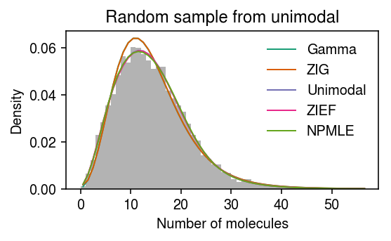
Take the fitted NPMLE \(\hat{g}\). For each observed \(x_{i+}\), draw one \(\lambda_i \sim \hat{g}\), then convolve with the measurement model.
np.random.seed(0)
g = np.array(unimodal_res.rx2('fitted_g'))
g = g[:,g[0] > 1e-8]
a = np.fmin(g[1], g[2])
b = np.fmax(g[1], g[2])
z = np.random.choice(g.shape[1], size=x.shape[0], p=g[0])
lam = np.random.uniform(a[z], b[z])
x = np.random.poisson(s * lam)
plt.clf()
plt.gcf().set_size_inches(4, 2.5)
plt.hist(x, bins=y, color='0.7', density=True, label=None)
for c, k in zip(plt.get_cmap('Dark2').colors, ['Gamma', 'ZIG', 'Unimodal', 'ZIEF', 'NPMLE']):
  plt.plot(y + .5, pmf[k], color=c, lw=1, label=k)
plt.legend(frameon=False)
plt.title('Random sample from unimodal')
plt.xlabel('Number of molecules')
plt.ylabel('Density')
plt.tight_layout()
Fit a dependent expression model.
def loss(a, x, s):
  return -np.array(scmodes.ebpm.ebpm_unimodal(x, np.exp(a * np.log(s))).rx2('loglik'))[0]

opt = so.minimize_scalar(loss, bracket=[0, 1], method='brent', args=(x, s))
assert opt.success
opt.x, opt.fun, -unimodal_res.rx2('loglik')[0]
(1.0177157921515285, 31202.115784911897, 31198.919049387503)
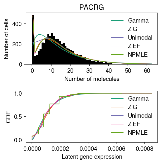
iPSC example
Pick a different, better-behaved example.
ipsc = anndata.read_h5ad('/project2/mstephens/aksarkar/projects/singlecell-ideas/data/ipsc/ipsc.h5ad')
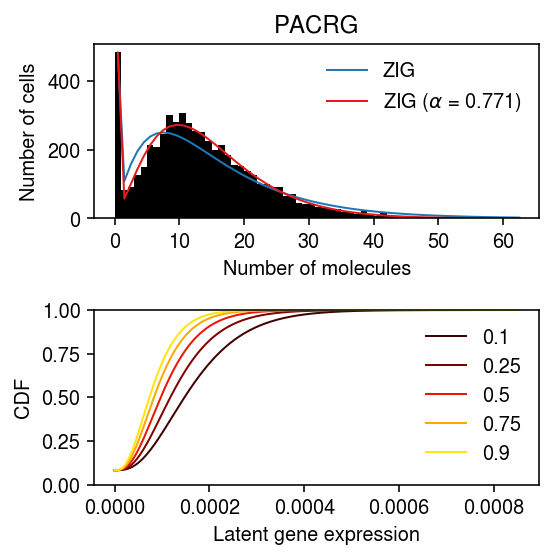
gene = 'PACRG'
x = ipsc[:,ipsc.var['name'] == gene].X.A.ravel()
s = ipsc.obs['mol_hs'].values.ravel()
y = np.arange(x.max() + 1)
grid = np.linspace(0, (x / s).max(), 1000)
pmf = dict()
erpp = dict()
cdf = dict()

gamma_res = scmodes.ebpm.ebpm_gamma(x, s)
pmf['Gamma'] = np.array([scmodes.benchmark.gof._zig_pmf(k, size=s, log_mu=gamma_res[0], log_phi=-gamma_res[1]).mean()
                         for k in y])
cdf['Gamma'] = st.gamma(a=np.exp(gamma_res[1]), scale=np.exp(gamma_res[0] - gamma_res[1])).cdf(grid)
erpp['Gamma'] = (scmodes.benchmark.gof._zig_cdf(x - 1, size=s, log_mu=gamma_res[0], log_phi=-gamma_res[1]) +
                 .5 * scmodes.benchmark.gof._zig_pmf(x, size=s, log_mu=gamma_res[0], log_phi=-gamma_res[1]))

point_gamma_res = scmodes.ebpm.ebpm_point_gamma(x, s)
cdf['ZIG'] = sp.expit(point_gamma_res[2]) + sp.expit(-point_gamma_res[2]) * st.gamma(a=np.exp(point_gamma_res[1]), scale=np.exp(point_gamma_res[0] - point_gamma_res[1])).cdf(grid)
pmf['ZIG'] = np.array([scmodes.benchmark.gof._zig_pmf(k, size=s, log_mu=point_gamma_res[0], log_phi=-point_gamma_res[1], logodds=point_gamma_res[2]).mean()
                       for k in y])
erpp['ZIG'] = (scmodes.benchmark.gof._zig_cdf(x - 1, size=s, log_mu=point_gamma_res[0], log_phi=-point_gamma_res[1], logodds=point_gamma_res[2]) +
               .5 * scmodes.benchmark.gof._zig_pmf(x, size=s, log_mu=point_gamma_res[0], log_phi=-point_gamma_res[1], logodds=-point_gamma_res[2]))

zief_res = scmodes.ebpm.ebpm_point_expfam(x, s)
pmf['ZIEF'] = np.array([scmodes.benchmark.gof._point_expfam_pmf(np.full(x.shape, k), size=s, res=zief_res).mean()
                        for k in y])
cdf['ZIEF'] = np.interp(grid, np.array(zief_res.slots['distribution'])[:,0], np.cumsum(np.array(zief_res.slots['distribution'])[:,1]))
erpp['ZIEF'] = (scmodes.benchmark.gof._point_expfam_cdf(x - 1, size=s, res=zief_res) +
                .5 * scmodes.benchmark.gof._point_expfam_pmf(x, size=s, res=zief_res))

unimodal_res = scmodes.ebpm.ebpm_unimodal(x, s)
g = np.array(unimodal_res.rx2('fitted_g'))
g = g[:,g[0] > 1e-8]
a = np.fmin(g[1], g[2])
b = np.fmax(g[1], g[2])
comp_dens_conv = np.array([((st.gamma(a=k + 1, scale=1 / s.reshape(-1, 1)).cdf(b.reshape(1, -1)) - st.gamma(a=k + 1, scale=1 / s.reshape(-1, 1)).cdf(a.reshape(1, -1))) / np.outer(s, b - a)).mean(axis=0) for k in y])
comp_dens_conv[:,0] = st.poisson(mu=s.reshape(-1, 1) * b[0]).pmf(y).mean(axis=0)
pmf['Unimodal'] = comp_dens_conv @ g[0]
cdf['Unimodal'] = ashr.cdf_ash(unimodal_res, grid).rx2('y').ravel()
erpp['Unimodal'] = (scmodes.benchmark.gof._ash_cdf(x - 1, s=s, fit=unimodal_res) +
                    .5 * scmodes.benchmark.gof._ash_pmf(x, s=s, fit=unimodal_res))

npmle_res = scmodes.ebpm.ebpm_npmle(x, s, step=1e-6)
g = np.array(npmle_res.rx2('fitted_g'))
g = g[:,g[0] > 1e-8]
a = np.fmin(g[1], g[2])
b = np.fmax(g[1], g[2])
comp_dens_conv = np.array([((st.gamma(a=k + 1, scale=1 / s.reshape(-1, 1)).cdf(b.reshape(1, -1)) - st.gamma(a=k + 1, scale=1 / s.reshape(-1, 1)).cdf(a.reshape(1, -1))) / np.outer(s, b - a)).mean(axis=0) for k in y])
pmf['NPMLE'] = comp_dens_conv @ g[0]
cdf['NPMLE'] = ashr.cdf_ash(npmle_res, grid).rx2('y').ravel()
erpp['NPMLE'] = (scmodes.benchmark.gof._ash_cdf(x - 1, s=s, fit=npmle_res) +
                 .5 * scmodes.benchmark.gof._ash_pmf(x, s=s, fit=npmle_res))
plt.clf()
fig, ax = plt.subplots(2, 1)
fig.set_size_inches(4, 4)
ax[0].hist(x, bins=y, color='k', label=None)
for c, k in zip(plt.get_cmap('Dark2').colors, ['Gamma', 'ZIG', 'Unimodal', 'ZIEF', 'NPMLE']):
  ax[0].plot(y + .5, x.shape[0] * pmf[k], color=c, lw=1, label=k)
ax[0].legend(frameon=False)
ax[0].set_title(gene)
ax[0].set_xlabel('Number of molecules')
ax[0].set_ylabel('Number of cells')

for c, k in zip(plt.get_cmap('Dark2').colors, ['Gamma', 'ZIG', 'Unimodal', 'ZIEF', 'NPMLE']):
  ax[1].plot(grid, cdf[k], color=c, lw=1, label=k)
ax[1].set_xlabel('Latent gene expression')
ax[1].set_ylabel('CDF')
ax[1].legend(frameon=False)
fig.tight_layout()
opt = so.minimize_scalar(lambda a: -scmodes.ebpm.ebpm_point_gamma(x, np.exp((1 - a) * np.log(s)))[-1], bracket=[0, 1])
opt
fun: 19321.753576794905
nfev: 16
nit: 12
success: True
x: 0.7713271091374253
point_gamma_res = scmodes.ebpm.ebpm_point_gamma(x, np.exp((1 - opt.x) * np.log(s)))
k = rf'ZIG ($\alpha$ = {opt.x:.3g})'
plt.clf()
fig, ax = plt.subplots(2, 1)
fig.set_size_inches(4, 4)
ax[0].hist(x, bins=y, color='k', label=None)
for c, k in zip(plt.get_cmap('Paired').colors, pmf):
  if k.startswith('ZIG'):
    ax[0].plot(y + .5, x.shape[0] * pmf[k], color=c, lw=1, label=k)
ax[0].legend(frameon=False)
ax[0].set_title(gene)
ax[0].set_xlabel('Number of molecules')
ax[0].set_ylabel('Number of cells')

for q in (.1, .25, .5, .75, .9):
  temp = np.percentile(sp.expit(point_gamma_res[2]) + sp.expit(-point_gamma_res[2]) * st.gamma(a=np.exp(point_gamma_res[1]), scale=np.exp(point_gamma_res[0] - point_gamma_res[1]) / np.exp(opt.x * np.log(s)).reshape(-1, 1)).cdf(grid), 100 * q, axis=0)
  ax[1].plot(grid, temp, color=colorcet.cm['fire'](q), lw=1, label=f'{q:.2g}')
ax[1].set_ylim(0, 1)
ax[1].set_xlabel('Latent gene expression')
ax[1].set_ylabel('CDF')
ax[1].legend(frameon=False)
fig.tight_layout()