Poisson-truncated normal data

Introduction
Setup
Example

Introduction

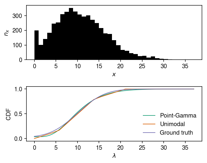
Zihao Wang shared an example simulated data set where ash gives a surprising result.

Setup

import numpy as np
import scipy.stats as st
import scmodes

%matplotlib inline
%config InlineBackend.figure_formats = set(['retina'])

import matplotlib.pyplot as plt
plt.rcParams['figure.facecolor'] = 'w'
plt.rcParams['font.family'] = 'Nimbus Sans'

Example

np.random.seed(1)
N = 5000
lam = np.clip(np.random.normal(loc=10, scale=5, size=N), 0, None)
x = np.random.poisson(lam=lam)
s = np.ones(x.shape)

grid = np.linspace(x.min(), x.max(), 1000)
F = st.norm(loc=10, scale=5)
true_cdf = F.cdf(0) + F.sf(0) * F.cdf(grid)

cm = plt.get_cmap('Dark2')
plt.clf()
fig, ax = plt.subplots(2, 1)
fig.set_size_inches(5, 4)

ax[0].hist(x, bins=np.arange(x.max() + 1), color='k')
ax[0].set_xlabel('$x$')
ax[0].set_ylabel('$n_x$')

for i, (method, t) in enumerate(zip(['zig', 'unimodal'], ['Point-Gamma', 'Unimodal'])):
  ax[1].plot(*getattr(scmodes.deconvolve, f'fit_{method}')(x, s), label=t, c=cm(i), lw=1)
ax[1].plot(grid, true_cdf, label='Ground truth', c=cm(2), lw=1)
ax[1].legend(frameon=False)
ax[1].set_xlabel('$\lambda$')
ax[1].set_ylabel('CDF')

fig.tight_layout()

The grid we used to parameterize the unimodal distribution is:

np.exp(np.arange(np.log(1 / s.mean()), np.log((x / s).max()), step=.5 * np.log(2)))

array([ 1.        ,  1.41421356,  2.        ,  2.82842712,  4.        ,
5.65685425,  8.        , 11.3137085 , 16.        , 22.627417  ,
32.        ])

Poisson-truncated normal data

Table of Contents

Introduction

Setup

Example