Poisson-Gamma log likelihood surface

Introduction
Setup
Results
- Likelihood surface for a simulated problem

Introduction

We previously implemented maximum likelihood estimation of the ZINB model

\begin{align*} x_{ij} \mid x_i^+, \lambda_{ij} &\sim \operatorname{Poisson}(x_i^+ \lambda_{ij})\\ \lambda_{ij} &\sim g_j(\cdot) = \pi_j \delta_0(\cdot) + (1 - \pi_j) \operatorname{Gamma}(1/\phi_j, 1/(\mu_j\phi_j)) \end{align*}

via batch gradient descent. We chose this algorithm because in the motivating application (variance QTL mapping; Sarkar et al. 2019):

The parameters \(\mu_j, \phi_j, \pi_j\) had a structure (one set of parameters per donor, per gene), resulting in >1.5 million parameters in total to be estimated from the data
Observed techncial covariates had effects which were shared across donors (due to randomization in the study design; this makes them estimable from the data, but complicates the model)
The algorithm is amenable to automatic differentiation and GPU computation

However, in our benchmarking for this study, this implementation has a major drawback: it requires memory on the order of the dimensions of the data. This is especially problematic for large, sparse data (e.g. 10X Genomics data). To address this problem, we have re-implemented this approach using stochastic gradient descent (in package scmodes). Here, we investigate convergence problems in this implementation.

Setup

import numpy as np
import scipy.stats as st
import scmodes.sgd
import scqtl.simple
import torch
import torch.utils.data

%matplotlib inline
%config InlineBackend.figure_formats = set(['retina'])

import colorcet
import matplotlib.pyplot as plt
plt.rcParams['figure.facecolor'] = 'w'
plt.rcParams['font.family'] = 'Nimbus Sans'

Results

Likelihood surface for a simulated problem

Simulate data for a single gene, fixing \(\pi_j = 0\) for simplicity.

np.random.seed(1)
# Typical values (Sarkar et al. 2019)
log_mu = np.random.uniform(-12, -6)
log_phi = np.random.uniform(-4, 0)

n = 5000
s = 1e5 * np.ones((n, 1))
lam = np.random.gamma(shape=np.exp(-log_phi), scale=np.exp(log_mu + log_phi), size=(n, 1))
x = np.random.poisson(lam=s * lam)

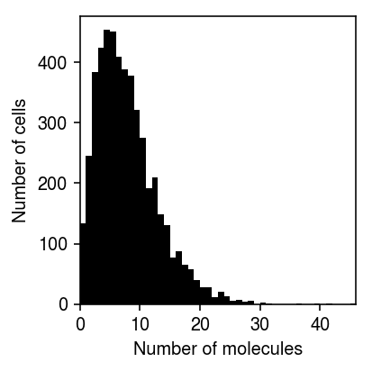
Plot the simulated data.

plt.clf()
plt.gcf().set_size_inches(3, 3)
plt.hist(x, bins=np.arange(x.max() + 1), color='k')
plt.xlim(0, x.max())
plt.xlabel('Number of molecules')
plt.ylabel('Number of cells')
plt.tight_layout()

Compute the log likelihood surface in a close window about the true value.

n_points = 100
window = 0.25
log_mu_grid = np.linspace(log_mu - window, log_mu + window, n_points)
log_phi_grid = np.linspace(log_phi - window, log_phi + window, n_points)
z = np.zeros((n_points, n_points))
for x_ in range(n_points):
  for y_ in range(n_points):
    z[y_, x_] = st.nbinom(n=np.exp(-log_phi_grid[y_]), p=1 / (1 + s * np.exp(log_mu_grid[x_] + log_phi_grid[y_]))).logpmf(x).sum()

Compute the MLE using the Nelder-Mead algorithm.

mu_hat, inv_phi_hat, _ = scqtl.simple.fit_nb(x.ravel(), s.ravel())

Trace the parameter values through batch gradient descent, starting from \(\ln\mu = 0, \ln\phi = 0\).

batch_gd_result = scmodes.sgd.ebpm_gamma(x, s, batch_size=n, max_epochs=2000, trace=True)

batch_trace_x = np.array(batch_gd_result[-1])[:,0]
batch_trace_y = -np.array(batch_gd_result[-1])[:,1]
batch_trace_keep = np.logical_and.reduce(
  (log_mu - window < batch_trace_x,
   batch_trace_x < log_mu + window,
   log_phi - window < batch_trace_y,
   batch_trace_y < log_phi + window))

Trace the parameter values through SGD, starting from \(\ln\mu = 0, \ln\phi = 0\).

# Important: learning rate needs to be reduced compared to batch gradient
# descent. (The default is 1e-2.)
sgd_result = scmodes.sgd.ebpm_gamma(x, s, batch_size=1, max_epochs=5, lr=1e-3, trace=True)

sgd_trace_x = np.array(sgd_result[-1])[:,0]
sgd_trace_y = -np.array(sgd_result[-1])[:,1]
sgd_trace_keep = np.logical_and.reduce(
  (log_mu - window < sgd_trace_x,
   sgd_trace_x < log_mu + window,
   log_phi - window < sgd_trace_y,
   sgd_trace_y < log_phi + window))

Trace the parameter values through minibatch SGD, starting from \(\ln\mu = 0, \ln\phi = 0\).

mb_sgd_result = scmodes.sgd.ebpm_gamma(x, s, batch_size=100, max_epochs=100, trace=True)

mb_sgd_trace_x = np.array(mb_sgd_result[-1])[:,0]
mb_sgd_trace_y = -np.array(mb_sgd_result[-1])[:,1]
mb_sgd_trace_keep = np.logical_and.reduce(
  (log_mu - window < mb_sgd_trace_x,
   mb_sgd_trace_x < log_mu + window,
   log_phi - window < mb_sgd_trace_y,
   mb_sgd_trace_y < log_phi + window))

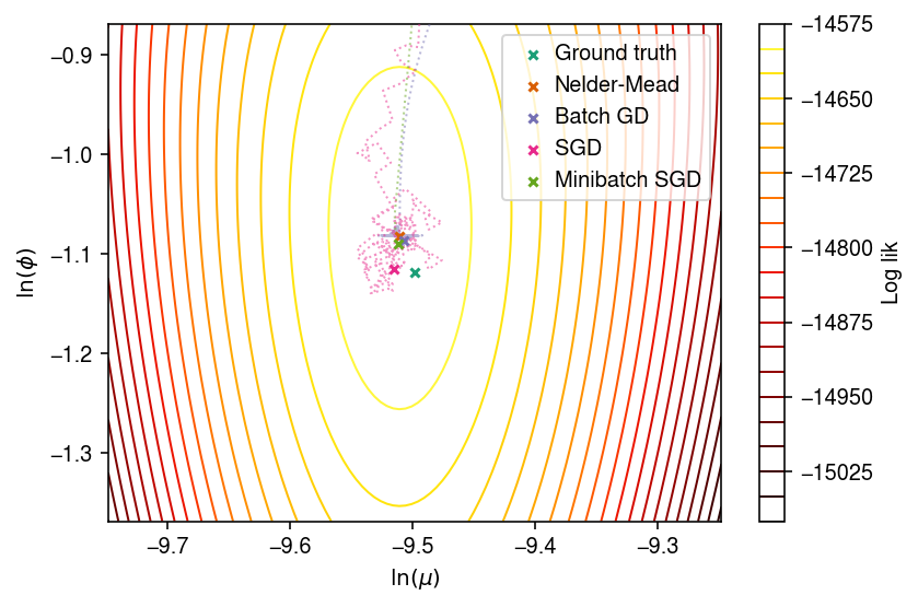
Plot the log likelihood surface and optimization traces.

cm = plt.get_cmap('Dark2')
plt.clf()
plt.gcf().set_size_inches(6, 4)
cf = plt.contour(log_mu_grid, log_phi_grid, z, levels=20, cmap=colorcet.cm['fire'], linewidths=1)
plt.scatter(log_mu, log_phi, marker='x', c=cm(0), s=16, zorder=10, label='Ground truth')
plt.scatter(np.log(mu_hat), -np.log(inv_phi_hat), marker='x', c=cm(1), s=16, zorder=10, label='Nelder-Mead')
plt.scatter(batch_gd_result[0], -batch_gd_result[1], marker='x', c=cm(2), s=16, zorder=10, label='Batch GD')
plt.scatter(sgd_result[0], -sgd_result[1], marker='x', c=cm(3), s=16, zorder=10, label='SGD')
plt.scatter(mb_sgd_result[0], -mb_sgd_result[1], marker='x', c=cm(4), s=16, zorder=10, label='Minibatch SGD')

plt.plot(batch_trace_x[batch_trace_keep], batch_trace_y[batch_trace_keep], c=cm(2), marker=None, ls=':', lw=1, alpha=0.5, zorder=4, label=None)
plt.plot(sgd_trace_x[sgd_trace_keep][::100], sgd_trace_y[sgd_trace_keep][::100], c=cm(3), marker=None, lw=1, ls=':', alpha=0.5, zorder=5, label=None)
plt.plot(mb_sgd_trace_x[mb_sgd_trace_keep][::100], mb_sgd_trace_y[mb_sgd_trace_keep][::100], c=cm(4), marker=None, lw=1, ls=':', alpha=0.5, zorder=5, label=None)

cb = plt.colorbar(cf)
cb.set_label('Log lik')
plt.legend(frameon=True, loc='best', handletextpad=0)
plt.xlabel('$\ln(\mu)$')
plt.ylabel('$\ln(\phi)$')
plt.tight_layout()

Poisson-Gamma log likelihood surface

Table of Contents

Introduction

Setup

Results

Likelihood surface for a simulated problem