Uniform vs half-uniform mixture prior

Introduction
Setup
Results
- iPSC example
- Chromium control data example

Introduction

We found cases where a unimodal expression model (half-uniform mixture) had a worse log likelihood than a Gamma expression model. This happened due to a bug in a previous version of ashr. Verify that it was fixed in version 2.2-51.

Setup

import anndata
import numpy as np
import pandas as pd
import scanpy as sc
import scmodes
import scipy.stats as st

import rpy2.robjects.packages
import rpy2.robjects.pandas2ri
rpy2.robjects.pandas2ri.activate()
ashr = rpy2.robjects.packages.importr('ashr')

%matplotlib inline
%config InlineBackend.figure_formats = set(['retina'])

import colorcet
import matplotlib
import matplotlib.pyplot as plt
plt.rcParams['figure.facecolor'] = 'w'
plt.rcParams['font.family'] = 'Nimbus Sans'

Results

iPSC example

dat = data['ipsc']()
x = dat[:,dat.var['index'] == 'ENSG00000013364'].X.A.ravel()
s = dat.obs['size'].values.ravel()

Fit candidate expression models, and report the log likelihood.

fit = {
  'Gamma': scmodes.ebpm.ebpm_gamma(x, s),
  'Unimodal (halfuniform)': scmodes.ebpm.ebpm_unimodal(x, s, mixcompdist='halfuniform'),
  'Unimodal (uniform)': scmodes.ebpm.ebpm_unimodal(x, s, mixcompdist='uniform'),
}

pd.Series({
  k: fit[k][-1] if isinstance(fit[k], tuple) else fit[k].rx2('loglik')[0]
  for k in fit
})

Gamma                    -4916.603271
Unimodal (halfuniform)   -4911.743860
Unimodal (uniform)       -4911.814471
dtype: float64

Look at the estimated unimodal models.

g0 = np.array(fit['Unimodal (uniform)'].rx2('fitted_g'))
g0[:,g0[0] > 1e-8]

array([[9.26309463e-01, 2.96562998e-02, 4.40342371e-02],
[9.24285849e-06, 0.00000000e+00, 0.00000000e+00],
[9.24285849e-06, 2.99375891e-05, 3.85096272e-05]])

g1 = np.array(fit['Unimodal (halfuniform)'].rx2('fitted_g'))
g1[:,0]

array([0.00000000e+00, 9.08008205e-06, 9.08008205e-06])

g1[:,g1[0] > 1e-8]

array([[4.53314869e-01, 4.74849764e-01, 5.27755773e-02, 1.90597899e-02],
[8.16422384e-06, 9.08008205e-06, 9.08008205e-06, 9.08008205e-06],
[9.08008205e-06, 9.72769161e-06, 2.98035879e-05, 3.83875450e-05]])

Look at the log likelihood as a function of the mode.

grid = np.linspace(0, 2e-5, 100)
llik0 = np.array([scmodes.ebpm.ebpm_unimodal(x, s, mixcompdist='uniform', mode=m).rx2('loglik')[0] for m in grid])
llik1 = np.array([scmodes.ebpm.ebpm_unimodal(x, s, mixcompdist='halfuniform', mode=m).rx2('loglik')[0] for m in grid])

cm = plt.get_cmap('Dark2')
plt.clf()
plt.gcf().set_size_inches(4, 2.5)
for i, (y, l) in enumerate(zip([llik0, llik1], ['Uniform', 'Half-uniform'])):
  plt.plot(grid, y, c=cm(i), label=l, lw=1)
  plt.axvline(grid[np.argmax(y)], c=cm(i), lw=1, ls=':', label=None)
plt.legend(frameon=False, loc='center left', bbox_to_anchor=(1, .5))
plt.xlabel('Mode')
plt.ylabel('Log likelihood')
plt.tight_layout()

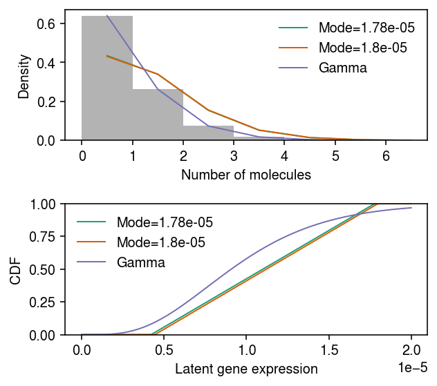
Look at the fits for two close choices of mode with very different log likelihoods.

fit0 = scmodes.ebpm.ebpm_unimodal(x, s, mixcompdist='halfuniform', mode=grid[88])
fit1 = scmodes.ebpm.ebpm_unimodal(x, s, mixcompdist='halfuniform', mode=grid[89])
pd.Series({
  f'{grid[88]:.3g}': fit0.rx2('loglik')[0],
  f'{grid[89]:.3g}': fit1.rx2('loglik')[0]
})

1.78e-05   -4930.230021
1.8e-05    -4936.446796
dtype: float64

pmf = dict()
y = np.arange(x.max() + 1)

g = np.array(fit0.rx2('fitted_g'))
g = g[:,g[0] > 1e-8]
a = np.fmin(g[1], g[2])
b = np.fmax(g[1], g[2])
comp_dens_conv = np.array([((st.gamma(a=k + 1, scale=1 / s.reshape(-1, 1)).cdf(b.reshape(1, -1)) - st.gamma(a=k + 1, scale=1 / s.reshape(-1, 1)).cdf(a.reshape(1, -1))) / np.outer(s, b - a)).mean(axis=0) for k in y])
comp_dens_conv[:,0] = st.poisson(mu=s.reshape(-1, 1) * b[0]).pmf(y).mean(axis=0)
pmf[grid[88]] = comp_dens_conv @ g[0]

g = np.array(fit1.rx2('fitted_g'))
g = g[:,g[0] > 1e-8]
a = np.fmin(g[1], g[2])
b = np.fmax(g[1], g[2])
comp_dens_conv = np.array([((st.gamma(a=k + 1, scale=1 / s.reshape(-1, 1)).cdf(b.reshape(1, -1)) - st.gamma(a=k + 1, scale=1 / s.reshape(-1, 1)).cdf(a.reshape(1, -1))) / np.outer(s, b - a)).mean(axis=0) for k in y])
comp_dens_conv[:,0] = st.poisson(mu=s.reshape(-1, 1) * b[0]).pmf(y).mean(axis=0)
pmf[grid[89]] = comp_dens_conv @ g[0]

cdf = dict()
temp = np.linspace(0, 2e-5, 1000)
cdf[grid[88]] = np.array(ashr.cdf_ash(fit0, temp).rx2('y')).ravel()
cdf[grid[89]] = np.array(ashr.cdf_ash(fit1, temp).rx2('y')).ravel()

cm = plt.get_cmap('Dark2')
plt.clf()
fig, ax = plt.subplots(2, 1)
fig.set_size_inches(4.5, 4)

temp = np.arange(x.max() + 1)
ax[0].hist(x, bins=temp, color='0.7', density=True)
for i, m in enumerate([88, 89]):
  ax[0].plot(temp + .5, pmf[grid[m]], lw=1, c=cm(i), label=f'Mode={grid[m]:.3g}')
gamma_res = scmodes.ebpm.ebpm_gamma(x, s)
ax[0].plot(temp + .5, np.array([scmodes.benchmark.gof._zig_pmf(k, size=s, log_mu=gamma_res[0], log_phi=-gamma_res[1]).mean() for k in temp]), lw=1, c=cm(2), label='Gamma')
ax[0].legend(frameon=False)
ax[0].set_xlabel('Number of molecules')
ax[0].set_ylabel('Density')

temp = np.linspace(0, 2e-5, 1000)
for i, m in enumerate([88, 89]):
  ax[1].plot(temp, cdf[grid[m]], lw=1, c=cm(i), label=f'Mode={grid[m]:.3g}')
ax[1].plot(temp, st.gamma(a=np.exp(gamma_res[1]), scale=np.exp(gamma_res[0] - gamma_res[1])).cdf(temp), lw=1, c=cm(2), label='Gamma')
ax[1].legend(frameon=False)
ax[1].set_ylim(0, 1)
ax[1].set_xlabel('Latent gene expression')
ax[1].set_ylabel('CDF')
fig.tight_layout()

Chromium control data example

dat = data['chromium1']()
x = dat[:,dat.var['index'] == 'ERCC-00024'].X.A.ravel()
s = dat.X.sum(axis=1).A.ravel()

fit = {
  'Gamma': scmodes.ebpm.ebpm_gamma(x, s),
  'Unimodal (halfuniform)': scmodes.ebpm.ebpm_unimodal(x, s, mixcompdist='halfuniform'),
  'Unimodal (uniform)': scmodes.ebpm.ebpm_unimodal(x, s, mixcompdist='uniform'),
}

pd.Series({
  k: fit[k][-1] if isinstance(fit[k], tuple) else fit[k].rx2('loglik')[0]
  for k in fit
})

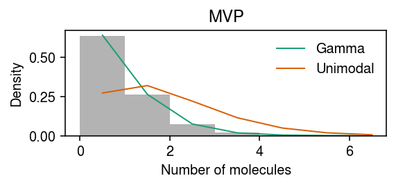
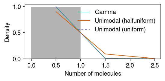
Gamma                     -45.478005
Unimodal (halfuniform)   -121.644443
Unimodal (uniform)        -45.460142
dtype: float64

pmf = dict()
y = np.arange(x.max() + 2)

pmf['Gamma'] = np.array([scmodes.benchmark.gof._zig_pmf(k, size=s, log_mu=fit['Gamma'][0], log_phi=-fit['Gamma'][1]).mean() for k in y])

g = np.array(fit['Unimodal (halfuniform)'].rx2('fitted_g'))
g = g[:,g[0] > 1e-8]
a = np.fmin(g[1], g[2])
b = np.fmax(g[1], g[2])
comp_dens_conv = np.array([((st.gamma(a=k + 1, scale=1 / s.reshape(-1, 1)).cdf(b.reshape(1, -1)) - st.gamma(a=k + 1, scale=1 / s.reshape(-1, 1)).cdf(a.reshape(1, -1))) / np.outer(s, b - a)).mean(axis=0) for k in y])
comp_dens_conv[:,0] = st.poisson(mu=s.reshape(-1, 1) * b[0]).pmf(y).mean(axis=0)
pmf['Unimodal (halfuniform)'] = comp_dens_conv @ g[0]

g = np.array(fit['Unimodal (uniform)'].rx2('fitted_g'))
g = g[:,g[0] > 1e-8]
a = np.fmin(g[1], g[2])
b = np.fmax(g[1], g[2])
comp_dens_conv = np.array([((st.gamma(a=k + 1, scale=1 / s.reshape(-1, 1)).cdf(b.reshape(1, -1)) - st.gamma(a=k + 1, scale=1 / s.reshape(-1, 1)).cdf(a.reshape(1, -1))) / np.outer(s, b - a)).mean(axis=0) for k in y])
comp_dens_conv[:,0] = st.poisson(mu=s.reshape(-1, 1) * b[0]).pmf(y).mean(axis=0)
pmf['Unimodal (uniform)'] = comp_dens_conv @ g[0]

cm = plt.get_cmap('Dark2')
plt.clf()
plt.gcf().set_size_inches(4, 2)
plt.hist(x, bins=y, color='0.7', density=True)
for i, (k, ls) in enumerate(zip(pmf, ['-', '-', (0, (3, 3))])):
  plt.plot(y + .5, pmf[k], lw=1, ls=ls, c=cm(i), label=k)
plt.legend(frameon=False)
plt.xlabel('Number of molecules')
plt.ylabel('Density')
plt.tight_layout()

Look at the fitted unimodal models.

g = np.array(fit['Unimodal (halfuniform)'].rx2('fitted_g'))
g[:,g[0] > 1e-8]

array([[1.00000000e+00],
[0.00000000e+00],
[7.55888146e-05]])

g = np.array(fit['Unimodal (uniform)'].rx2('fitted_g'))
g[:,g[0] > 1e-8]

array([[1.0000000e+00],
[2.5777149e-06],
[2.5777149e-06]])

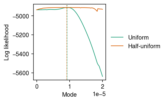
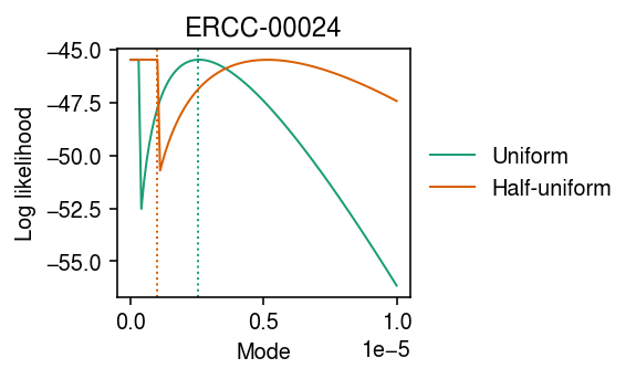
Look at the mode search.

grid = np.linspace(0, 1e-5, 100)
llik0 = np.array([scmodes.ebpm.ebpm_unimodal(x, s, mixcompdist='uniform', mode=m).rx2('loglik')[0] for m in grid])
llik1 = np.array([scmodes.ebpm.ebpm_unimodal(x, s, mixcompdist='halfuniform', mode=m).rx2('loglik')[0] for m in grid])

cm = plt.get_cmap('Dark2')
plt.clf()
plt.gcf().set_size_inches(4, 2.5)
for i, (y, l) in enumerate(zip([llik0, llik1], ['Uniform', 'Half-uniform'])):
  plt.plot(grid, y, c=cm(i), label=l, lw=1)
  plt.axvline(grid[np.argmax(y)], c=cm(i), lw=1, ls=':', label=None)
plt.legend(frameon=False, loc='center left', bbox_to_anchor=(1, .5))
plt.xlabel('Mode')
plt.ylabel('Log likelihood')
plt.title('ERCC-00024')
plt.tight_layout()

Look at the mode search over a larger range (coarser grid) of candidate modes.

grid = np.linspace(0, 1e-4, 100)
llik0 = np.array([scmodes.ebpm.ebpm_unimodal(x, s, mixcompdist='uniform', mode=m).rx2('loglik')[0] for m in grid])
llik1 = np.array([scmodes.ebpm.ebpm_unimodal(x, s, mixcompdist='halfuniform', mode=m).rx2('loglik')[0] for m in grid])

cm = plt.get_cmap('Dark2')
plt.clf()
plt.gcf().set_size_inches(4, 2.5)
for i, (y, l) in enumerate(zip([llik0, llik1], ['Uniform', 'Half-uniform'])):
  plt.plot(grid, y, c=cm(i), label=l, lw=1)
  plt.axvline(grid[np.argmax(y)], c=cm(i), lw=1, ls=':', label=None)
plt.legend(frameon=False, loc='center left', bbox_to_anchor=(1, .5))
plt.xlabel('Mode')
plt.ylabel('Log likelihood')
plt.title('ERCC-00024')
plt.tight_layout()

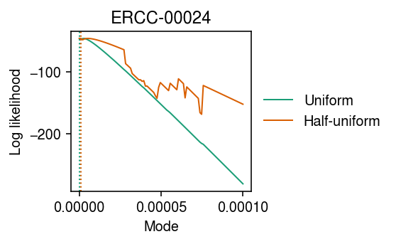
Find points where the log likelihood does not decrease monotonically with moving the candidate mode further from the optimum.

np.where(np.diff(llik1) > 0)

(array([ 0,  2,  3,  4, 36, 38, 40, 47, 48, 54, 59, 64, 74]),)

pd.Series({
  grid[k]: llik1[k]
   for k in (47, 48)
})

0.000047   -142.753761
0.000048   -124.794312
dtype: float64

Look at the effect of changing the granularity of the grid (tuning gridmult) on the solution.

dat <- readRDS('/scratch/midway2/aksarkar/modes/chromium1-ERCC-00024.Rds')
x <- dat$x
s <- dat$s
print(ashr::ash_pois(x, s, mixcompdist='halfuniform', control=list(tol.svd=0), outputlevel='loglik')$loglik, digits=12)

opt <- stats::optimize(
  function (mode) {
    stats::optimize(
      function(gridmult) {
        -ashr::ash_pois(x, s, mixcompdist='halfuniform', mode=mode, gridmult=gridmult, outputlevel='loglik', control=list(tol.svd=0))$loglik
      },
      interval=c(1, 2),
      tol=1e-2)$objective
  },
  interval=c(0, max(x / s)),
  tol=max(x / s) * .Machine$double.eps^0.25)
print(opt, digits=12)

source activate scmodes
srun --partition=mstephens R --quiet --no-save <<'EOF'
<<nested-opt>>
EOF

> dat <- readRDS('/scratch/midway2/aksarkar/modes/chromium1-ERCC-00024.Rds')
> x <- dat$x
> s <- dat$s
> print(ashr::ash_pois(x, s, mixcompdist='halfuniform', control=list(tol.svd=0), outputlevel='loglik')$loglik, digits=12)
[1] -121.636120776
> 
> opt <- stats::optimize(
+   function (mode) {
+     stats::optimize(
+       function(gridmult) {
+         -ashr::ash_pois(x, s, mixcompdist='halfuniform', mode=mode, gridmult=gridmult, outputlevel='loglik', control=list(tol.svd=0))$loglik
+       },
+       interval=c(1, 2),
+       tol=1e-2)$objective
+   },
+   interval=c(0, max(x / s)),
+   tol=max(x / s) * .Machine$double.eps^0.25)
> print(opt, digits=12)
$minimum
[1] 5.13581372547e-06

$objective
[1] 45.4661257195

>

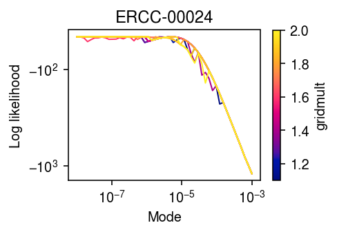
Check whether the log likelihood varies smoothly with gridmult.

modes = np.logspace(-8, -3, 50)
gridmults = np.linspace(1.1, 2, 10)
llik = np.array([[scmodes.ebpm.ebpm_unimodal(x, s, mixcompdist='halfuniform', mode=m, gridmult=gm).rx2('loglik')[0]
                  for m in modes]
                 for gm in gridmults])

cm = colorcet.cm['bmy']
plt.clf()
plt.gcf().set_size_inches(3.5, 2.5)
plt.xscale('log')
plt.yscale('symlog')
for gm, l in zip(gridmults, llik):
  plt.plot(modes, l, c=cm((gm - 1.1) / (2 - 1.1)), lw=1)
cb = plt.colorbar(matplotlib.cm.ScalarMappable(matplotlib.colors.Normalize(vmin=1.1, vmax=2), cmap=cm))
cb.set_label('gridmult')
plt.xlabel('Mode')
plt.ylabel('Log likelihood')
plt.title('ERCC-00024')
plt.tight_layout()