Gamma deconvolution

Introduction
Setup
Results

Introduction

Deconvolution assuming Gamma or point-Gamma latent gene expression distribution does worse than expected. Investigate why by comparing different implementations on an example problem.

Setup

import numpy as np
import pandas as pd
import rpy2.robjects
import rpy2.robjects.packages
import rpy2.robjects.pandas2ri
import scipy.special as sp
import scipy.stats as st
import scmodes
import scqtl
import scqtl.simple

rpy2.robjects.pandas2ri.activate()
pscl = rpy2.robjects.packages.importr('pscl')

%matplotlib inline
%config InlineBackend.figure_formats = set(['retina'])

import matplotlib.pyplot as plt
plt.rcParams['figure.facecolor'] = 'w'
plt.rcParams['font.family'] = 'Nimbus Sans L'

Results

Simulation

Simulate a simple example.

np.random.seed(4)
N = 1000
s = 1e5 * np.ones(N)
mu = 1e-3
# Inverse dispersion = 3
u = st.gamma(a=3, scale=1/3).rvs(size=N)
z = (np.random.uniform(size=N) < 0.95).astype(float)
x = np.random.poisson(lam=s * mu * u * z)

Report the logit-transformed size of the point mass on zero.

sp.logit(0.05)

-2.9444389791664403

Simple CPU implementation

We implemented Gamma deconvolution using the Nelder-Mead algorithm in the scqtl package.

res = scqtl.simple.fit_zinb(x, s)
pd.Series(res, index=['mean', 'inv_disp', 'logodds', 'llik'])

mean           0.000999
inv_disp       3.097253
logodds       -2.924002
llik       -5284.263660
dtype: float64

Political Science Computation Laboratory implementation

The R package pscl contains a function zeroinfl for fitting zero-inflated generalized linear models. We can write simple deconvolution problems in this form.

def pscl_zinb(x, s):
  f = rpy2.robjects.Formula('x ~ offset(log(s)) + 1 | 1')
  f.environment['x'] = x
  f.environment['s'] = s
  res = pscl.zeroinfl(f, dist='negbin')
  mean = np.exp(np.array(res.rx2('coefficients').rx2('count')))
  inv_disp = np.array(res.rx2('theta'))
  logodds = np.array(res.rx2('coefficients').rx2('zero'))
  llik = np.array(res.rx2('loglik'))
  return pd.Series(np.concatenate([mean, inv_disp, logodds, llik]), index=['mean', 'inv_disp', 'logodds', 'llik'])

pscl_zinb(x, s)

mean           0.000999
inv_disp       3.097312
logodds       -2.923963
llik       -5284.263659
dtype: float64

Looking at the implementation, there appear to be three major differences:

Comparison of CPU/GPU implementation on real data

We previously fit point-Gamma distributions to the latent gene expression of sorted CD8+ T cells from Zheng et al. 2017.

Read the GPU-fitted results.

gpu_log_mu = pd.read_csv('/project2/mstephens/aksarkar/projects/singlecell-modes/data/deconv-example/zheng-cd8-zinb-log-mu.txt.gz', sep='\t', index_col=0)
gpu_log_phi = pd.read_csv('/project2/mstephens/aksarkar/projects/singlecell-modes/data/deconv-example/zheng-cd8-zinb-log-phi.txt.gz', sep='\t', index_col=0)
gpu_logodds = pd.read_csv('/project2/mstephens/aksarkar/projects/singlecell-modes/data/deconv-example/zheng-cd8-zinb-logodds.txt.gz', sep='\t', index_col=0)

Compute the log likelihood of the GPU solution.

x = scmodes.dataset.read_10x('/project2/mstephens/aksarkar/projects/singlecell-ideas/data/10xgenomics/cytotoxic_t/filtered_matrices_mex/hg19')
s = x.sum(axis=1)

gpu_nb_llik = np.array([st.nbinom(n=np.exp(-log_phi), p=1/(1 + s * np.exp(log_mu + log_phi))).logpmf(x_j) for log_mu, log_phi, x_j in zip(gpu_log_mu.values.T, gpu_log_phi.values.T, x.T)])
case_zero = -np.log1p(np.exp(-gpu_logodds.values.T)) + np.log1p(np.exp(gpu_nb_llik - gpu_logodds.values.T))
case_nonzero = -np.log1p(np.exp(gpu_logodds.values.T)) + gpu_nb_llik
gpu_zinb_llik = np.where(x.T < 1, case_zero, case_nonzero)

Write out the GPU results.

gpu_res = pd.DataFrame({'mean': np.exp(gpu_log_mu.values.ravel()),
                        'inv_disp': np.exp(-gpu_log_phi.values.ravel()),
                        'logodds': gpu_logodds.values.ravel(),
                        'llik': gpu_zinb_llik.sum(axis=1)})
gpu_res.to_csv('/project2/mstephens/aksarkar/projects/singlecell-modes/data/gamma-deconv/gpu.txt.gz', sep='\t', compression='gzip')

Run CPU methods.

def fit_all(x, s, method):
  res = []
  for j in range(x.shape[1]):
    try:
      res.append(method(x[:,j], s))
    except:
      # Failed to converge
      res.append(np.array([np.nan, np.nan, np.nan, np.nan]))
  return pd.DataFrame(res, columns=['mean', 'inv_disp', 'logodds', 'llik'])

scqtl_res = fit_all(x, s, scqtl.simple.fit_zinb)
scqtl_res.to_csv('/project2/mstephens/aksarkar/projects/singlecell-modes/data/gamma-deconv/scqtl.txt.gz', sep='\t', compression='gzip')

pscl_res = fit_all(x, s, pscl_zinb)
pscl_res.to_csv('/project2/mstephens/aksarkar/projects/singlecell-modes/data/gamma-deconv/pscl.txt.gz', sep='\t', compression='gzip')

Read the results.

gpu_res = pd.read_csv('/project2/mstephens/aksarkar/projects/singlecell-modes/data/gamma-deconv/gpu.txt.gz', sep='\t')
pscl_res = pd.read_csv('/project2/mstephens/aksarkar/projects/singlecell-modes/data/gamma-deconv/pscl.txt.gz', sep='\t')
scqtl_res = pd.read_csv('/project2/mstephens/aksarkar/projects/singlecell-modes/data/gamma-deconv/scqtl.txt.gz', sep='\t')

Plot the difference in (training) log likelihood.

T = pd.DataFrame({'gpu': gpu_res['llik'],
                  'cpu': scqtl_res['llik'],
                  'pscl': pscl_res['llik']}).dropna()

plt.clf()
plt.gcf().set_size_inches(3, 3)
plt.boxplot((T.values - T['gpu'].values.reshape(-1, 1))[:,1:] / x.shape[0],
            medianprops={'color': 'k'}, flierprops={'marker': '.', 'markersize': 4})
plt.xticks(range(1, 3), T.columns[1:])
plt.xlabel('Method')
plt.ylabel('Per obs diff train llik from GPU')
plt.tight_layout()

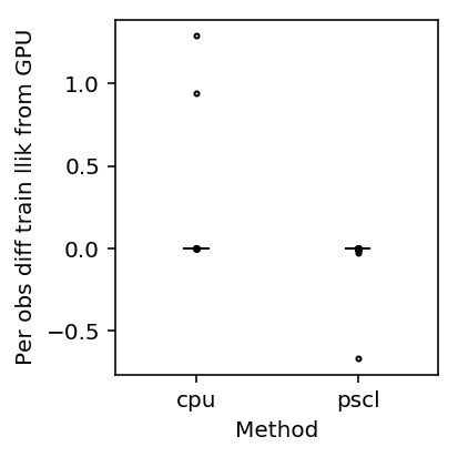
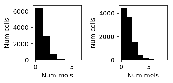
Look at cases where CPU does much better than GPU.

llik_diff = T['cpu'] - T['gpu']
query = llik_diff[llik_diff / x.shape[0] > 0.5].index

plt.clf()
fig, ax = plt.subplots(1, 2)
fig.set_size_inches(4, 2)
for a, k in zip(ax, query):
  a.hist(x[:,k], color='k', bins=np.arange(x[:,k].max() + 1))
  a.set_xlabel('Num mols')
  a.set_ylabel('Num cells')
fig.tight_layout()

Inspect the GPU result.

gpu_res.iloc[query]

mean     inv_disp    logodds          llik
25   0.000358  1164.383452 -12.345718  -9030.897929
377  0.000647   990.383954 -13.082376 -12151.227973

Inspect the CPU result.

scqtl_res.iloc[query]

mean      inv_disp   logodds         llik
25   0.000356  2.852713e+14 -8.394238   610.494460
377  0.000645  2.852848e+14 -8.395699  1006.905231

The results suggest the log likelihood computation had a numerical problem. Check against a Poisson model.

pd.DataFrame([scqtl.simple.fit_pois(xj, s) for xj in x[:,query].T], columns=['mean', 'llik'])

mean          llik
0  0.000358  -9030.866338
1  0.000647 -12151.180012

Check our implementation of ZINB log likelihood.

scmodes.benchmark.deconvolution.zinb_llik(x, s.reshape(-1, 1) * gpu_res['mean'].values, gpu_res['inv_disp'].values, gpu_res['logodds'].values).sum(axis=0)[query]

array([ -9030.89792855, -12151.22797265])