Poisson-unimodal Gamma mixture model

Introduction
Setup
Methods
- Unimodal mixture of Gammas
- Expectation-maximization algorithm
Results
- Tracing line search
- Test derivative implementation

Introduction

We have previously investigated the use of the following model for scRNA-seq counts coming from a single gene:

\begin{align*} x_{ij} &\sim \operatorname{Poisson}(x_i^+ \lambda_{ij})\\ \lambda_{ij} &\sim g_j(\cdot) = \sum_k \pi_{jk} \operatorname{Uniform}(\cdot; \lambda_{0j}, a_{jk}) \end{align*}

where \(x_i^+ = \sum_j x_{ij}\) and we abuse notation to allow \(a_{jk} < \lambda_{0j}\). In this model, expression variation is assumed to follow a unimodal non-parametric distribution \(g_j(\cdot)\), approximated as a large, but finite mixture of uniforms. The main challenge in fitting this model is estimating \(\lambda_{0j}\) (with \(\lambda_{0j}\) known, estimating \(g_j\) is a convex optimization problem solved by mixsqp). The strategy taken in ashr is to treat the mixsqp problem as a subroutine in line search over \(\lambda_{0j}\).

Here, we investigate using a unimodal mixture of Gammas (previously considered in Lu & Stephens 2016), which is a slightly less flexible assumption on expression variation, but could allow faster mode estimation.

Setup

import numpy as np
import pandas as pd
import rpy2.robjects.packages
import rpy2.robjects.pandas2ri
import scipy.optimize as so
import scipy.special as sp
import scipy.stats as st

ashr = rpy2.robjects.packages.importr('ashr')
mixsqp = rpy2.robjects.packages.importr('mixsqp')
rpy2.robjects.pandas2ri.activate()

%matplotlib inline
%config InlineBackend.figure_formats = set(['retina'])

import matplotlib.pyplot as plt
plt.rcParams['figure.facecolor'] = 'w'
plt.rcParams['font.family'] = 'Nimbus Sans'

Methods

Unimodal mixture of Gammas

Consider \(\lambda \sim \operatorname{Gamma}(\alpha, \beta)\). Let \(\lambda_0 = (\alpha - 1) / \beta\) (the mode), and \(v = \alpha / \beta^2\) (the variance). Then,

\begin{align*} \beta &= \frac{\lambda_0 + \sqrt{\lambda_0^2 + 4 v}}{2 v}\\ \alpha &= \lambda_0 \frac{\lambda_0 + \sqrt{\lambda_0^2 + 4 v}}{2 v} + 1 \end{align*}

and for choice of mode \(\lambda_{0j}\) and grid of variances \(v_{j1}, \ldots, v_{jK}\) we have

\[ \lambda_{ij} \sim g_j(\cdot) = \sum_{k=1}^K \pi_{jk} \operatorname{Gamma}(\cdot; \alpha_{jk}, \beta_{jk}) \]

As an illustrative example,

lam0 = 1e-3
# 1/s -> max(x/s)
mixvar = np.exp(np.arange(np.log(1 / 1e5), np.log(5e-3), step=.5 * np.log(2)))
grid = np.linspace(0, 1e-2, 1000)

cm = plt.get_cmap('Paired')
plt.clf()
plt.gcf().set_size_inches(3, 3)
for i, v in enumerate(mixvar[:5]):
  b = (lam0 + np.sqrt(lam0 * lam0 + 4 * v)) / (2 * v)
  a = lam0 * b + 1
  plt.plot(grid, st.gamma(a=a, scale=1 / b).pdf(grid), lw=1, c=cm(i))
plt.axvline(x=lam0, c='r', ls=':', lw=1)
plt.xlabel('$\lambda$')
plt.ylabel('$f(\lambda)$')
plt.tight_layout()

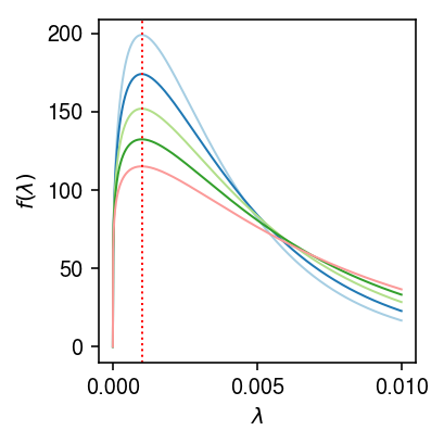
The main advantage of assuming a mixture of Gammas is that the marginal likelihood of \(x_{ij}\) is then a mixture of Negative Binomial distributions

\[ p(x_{1j}, \ldots, x_{nj} \mid x_1^+, \ldots, x_n^+, g) = \prod_i \sum_k \pi_{jk} \operatorname{NB}(x_{ij}; \alpha_{jk}, \frac{x_i^+}{x_i^+ + \beta_{jk}}). \]

Expectation-maximization algorithm

Introduce indicator variable \(z_i \in \{1, \ldots, K\}\) denoting which component \(\lambda_i\) was drawn from (dropping index \(j\)), and let \(\zeta_{ik} = p(z_i = k \mid x_i, x_i^+, g)\). Then

\begin{multline*} l(\cdot) = \sum_i E_{z_i \mid x_i, x_i^+, g}[\ln p(x_i, z_i \mid x_i^+, g)] = \\ \sum_{i, k} \zeta_{ik} \left( \ln \pi_k + x_i \ln\left(\frac{x_i^+}{x_i^+ + \beta_k}\right) + \alpha_k \ln\left(\frac{\beta_k}{x_i^+ + \beta_k}\right) + \ln\Gamma(x_i + \alpha_k) - \ln\Gamma(x_i + 1) - \ln\Gamma(\alpha_k) \right) \end{multline*}

suggesting an EM algorithm:

E step:

\[ \zeta_{ik} \propto \pi_k \operatorname{NB}(x_{ij}; \alpha_{k}, \frac{x_i^+}{x_i^+ + \beta_{k}}) \]

M step:

Update \(\boldsymbol\pi\) (solution to mixsqp)
Update \(\lambda_0\) (e.g. backtracking line search in direction of the gradient):
\begin{align*} \frac{\partial l}{\partial \alpha_k} &= \sum_i \zeta_{ik}\left( \ln\left(\frac{\beta_k}{x_i^+ + \beta_k}\right) + \psi(x_i + \alpha_k) - \psi(\alpha_k) \right)\\ \frac{\partial l}{\partial \beta_k} &= \sum_i \zeta_{ik} \left(\frac{\alpha_k}{\beta_k} - \frac{x_i + \alpha_k}{x_i^+ + \beta_k}\right)\\ \frac{\partial \alpha_k}{\partial \beta_k} &= \lambda_0\\ \frac{\partial \alpha_k}{\partial \lambda_0} &= \beta_k\\ \frac{\partial \beta_k}{\partial \lambda_0} &= \frac{1}{2 v} + \frac{\lambda_0}{2 v \sqrt{\lambda_0^2 + 4 v}} \end{align*}
where \(\psi\) denotes the digamma function.

def pois_gammamix_dlam0(x, s, a, b, zeta, lam0):
  """Return derivative of expected log joint wrt lam0, evaluated at current
values"""
  # Important: x, s are (n, 1); a, b, pi are (1, m); zeta is (n, m)
  a = a.reshape(1, -1)
  b = b.reshape(1, -1)
  # (1, m)
  dl_da = (zeta * (np.log(b) - np.log(s + b) + sp.digamma(x + a) - sp.digamma(a))).sum(axis=0, keepdims=True)
  dl_db = (zeta * (a / b - (x + a) / (s + b))).sum(axis=0, keepdims=True)
  v = a / (b * b)
  db_dlam = 1 / (2 * v) + lam0 / (2 * v * np.sqrt(lam0 ** 2 + 4 * v))
  da_dlam = lam0 * db_dlam + b
  # (1, 1)
  res = dl_da.dot(da_dlam.T) + dl_db.dot(db_dlam.T)
  return res[0, 0]

def pois_gammamix_obj(x, s, a, b, pi, zeta):
  """Return expected log joint"""
  # Important: x, s are (n, 1); a, b, pi are (1, m); zeta is (n, m)
  a = a.reshape(1, -1)
  b = b.reshape(1, -1)
  pi = pi.reshape(1, -1)
  return (zeta * (np.log(pi)
                  + x * np.log(s)
                  + a * np.log(b)
                  - (x + a) * np.log(s + b)
                  + sp.gammaln(x + a)
                  - sp.gammaln(x + 1)
                  - sp.gammaln(a))).sum()

def pois_gammamix_em(x, s, max_iter=100):
  lam_hat = x / s
  # Initialization
  lam0 = np.median(lam_hat)
  for i in range(max_iter):
    # Update pi
    mixvar = np.exp(np.arange(np.log(1 / s.median()), np.log(lam_hat.max()), step=.5 * np.log(2)))
    b = (lam0 + np.sqrt(lam0 * lam0 + 4 * mixvar)) / (2 * mixvar)
    a = lam0 * b + 1
    llik = st.nbinom(n=a, p=s / (s + b)).logpmf(x.reshape(-1, 1))
    mixsqp_res = mixsqp.mixsqp(pd.DataFrame(llik), log=True)
    pi = np.array(mixsqp_res.rx2('x'))
    # Update zeta
    zeta = pi.dot(np.exp(llik - llik.max()))
    zeta /= zeta.sum()
    # Update lam0

Results

Tracing line search

Trace how many function evaluations are used in estimating the mode, by writing a Python wrapper which can be called from scipy.optimize. (R stats::optimize does not return the number of function evaluations.)

def _ash(mode, x, s):
  """Return negative log likelihood of x, s given mode"""
  if mode < 0:
    return np.inf
  return -np.array(ashr.ash(
    pd.Series(np.zeros(n)),
    1,
    lik=ashr.lik_pois(y=pd.Series(x), scale=pd.Series(s), link='identity'),
    mixcompdist='halfuniform',
    outputlevel='loglik',
    mode=mode).rx2('loglik'))

def trial(n, disp=None, seed=0):
  np.random.seed(seed)
  n = n
  s = np.random.poisson(lam=1e4, size=n)
  mu = np.random.lognormal(mean=np.log(1e-4))
  if disp is None:
    x = np.random.poisson(lam=s * mu)
  elif disp <= 0:
    raise ValueError('disp must be > 0')
  else:
    x = np.random.negative_binomial(n=1 / disp, p=s * mu / (s * mu + 1 / disp))
  res = so.minimize_scalar(_ash, bracket=[(x / s).min(), (x / s).max()], args=(x, s), method='brent')
  if not res.success:
    raise RuntimeError(f'failed to converge: ')
  return res.nfev

Look at the number of function evaluations for one problem.

trial(n=100, seed=0)

Look at the mean and standard deviation of the number of function evaluations over multiple simulated problems, as a function of sample size \(n\).

nfev = []
n_trials = 5
for n in (100, 500, 1000):
  for i in range(n_trials):
    nfev.append((n, i, trial(n=n, seed=i)))
nfev = pd.DataFrame(nfev, columns=['n', 'trial', 'nfev'])
nfev.groupby(['n'])['nfev'].agg([np.mean, np.std])

mean       std
n
100   29.2  3.834058
500   28.2  3.271085
1000  25.4  6.730527

Repeat the benchmark for Poisson-Gamma distributed data.

nfev_nb = []
n_trials = 5
for n in (100, 500, 1000):
  for phi in (0.1, 0.3, 0.5):
    for i in range(n_trials):
      nfev_nb.append((n, phi, i, trial(n=n, disp=phi, seed=i)))
nfev_nb = pd.DataFrame(nfev_nb, columns=['n', 'phi', 'trial', 'nfev'])

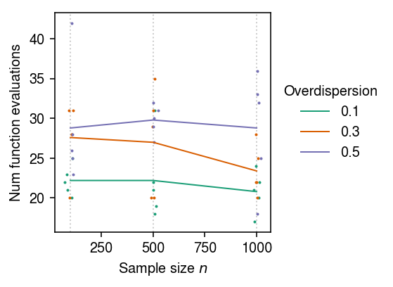
Plot the mean and standard deviation of the number of function evaluations for Poisson-Gamma problems as a function of sample size \(n\) and overdispersion \(\phi\).

cm = plt.get_cmap('Dark2')
plt.clf()
plt.gcf().set_size_inches(4, 3)
for n in (100, 500, 1000):
  plt.axvline(x=n, c='0.8', lw=1, ls=':', zorder=0)
for i, (k, g) in enumerate(nfev_nb.groupby(['phi'])):
  h = g.groupby('n')['nfev'].agg([np.mean, np.std]).reset_index()
  plt.plot(h['n'], h['mean'], ls='-', lw=1, c=cm(i), label=k)
  plt.scatter(x=g['n'] + np.random.normal(scale=10, size=g.shape[0]), y=g['nfev'], s=1, c=np.atleast_2d(cm(i)), label=None)
plt.xlabel('Sample size $n$')
plt.ylabel('Num function evaluations')
plt.legend(frameon=False, title='Overdispersion', loc='center left', bbox_to_anchor=(1, .5))
plt.tight_layout()

Test derivative implementation

Simulate some data.

np.random.seed(1)
n = 100
s = np.random.poisson(lam=1e4, size=n).reshape(-1, 1)
mu = 1e-4
x = np.random.poisson(lam=s * mu)

Pick some parameters.

lam_hat = x / s
lam0 = np.median(lam_hat)
mixvar = np.exp(np.arange(np.log(1 / np.median(s)), np.log(lam_hat.max()), step=.5 * np.log(2)))
b = (lam0 + np.sqrt(lam0 * lam0 + 4 * mixvar)) / (2 * mixvar)
a = lam0 * b + 1
pi = np.ones(mixvar.shape[0]) / mixvar.shape[0]
llik = st.nbinom(n=a.reshape(1, -1), p=s / (s + b.reshape(1, -1))).logpmf(x.reshape(-1, 1))
zeta = np.exp(llik - llik.max(axis=1, keepdims=True)) * pi
zeta /= zeta.sum(axis=1, keepdims=True)

Test the implementation of the derivative by fuzzing.

f0 = pois_gammamix_obj(x, s, a, b, pi, zeta)
df_dlam0 = pois_gammamix_dlam0(x, s, a, b, zeta, lam0)
eps = np.random.normal(scale=1e-5)
new_lam0 = lam0 + eps
new_b = (new_lam0 + np.sqrt(new_lam0 * new_lam0 + 4 * mixvar)) / (2 * mixvar)
new_a = new_lam0 * b + 1
new_f = pois_gammamix_obj(x, s, new_a, new_b, pi, zeta)
h = (new_f - f0) / eps
df_dlam0, h

(-26951.309882979232, -26828.742108484763)