Negative binomial measurement model
Table of Contents
Introduction
We, and Svensson 2020, found some evidence for overdispersion in control scRNA-seq data. Here, we estimate to what extent that overdispersion could be explained by an overdispersed measurement model, using the key fact that the measurement overdispersion is described by a single parameter common across all genes. We specifically consider combining an NB measurement model with a Gamma expression model \( \DeclareMathOperator\Pois{Poisson} \DeclareMathOperator\Gam{Gamma} \DeclareMathOperator\NB{NB} \DeclareMathOperator\V{V} \newcommand\const{\mathrm{const}} \newcommand\lnb{l_{\mathrm{NB}}} \newcommand\E[1]{\left\langle #1 \right\rangle} \)
\begin{align} x_{ij} \mid s_i, \lambda_{ij}, u_{ij} &\sim \NB(s_i \lambda_{ij}, \theta)\\ \lambda_{ij} \mid a_j, b_j &\sim \Gam(a_j, b_j), \end{align}where the NB distribution is parameterized by mean and dispersion, and the Gamma distribution is parameterized by shape and rate.
Setup
import numpy as np
import pandas as pd
import pickle
import scanpy as sc
import scipy.optimize as so
import scipy.special as sp
import scipy.stats as st
import scmodes
%matplotlib inline
%config InlineBackend.figure_formats = set(['retina'])
import colorcet
import matplotlib
import matplotlib.pyplot as plt
plt.rcParams['figure.facecolor'] = 'w'
plt.rcParams['font.family'] = 'Nimbus Sans'
Results
Simulate from the NB measurement model
Simulate data from the model.
def simulate_nb_gamma(n, p, theta, seed=0):
  np.random.seed(seed)
  log_mean = np.random.uniform(low=-12, high=-8, size=(1, p))
  log_disp = np.random.uniform(low=-6, high=0, size=(1, p))
  s = 1e5 * np.ones((n, 1))
  lam = st.gamma(a=np.exp(-log_disp), scale=np.exp(log_mean + log_disp)).rvs(size=(n, p))
  if theta > 0:
    u = st.gamma(a=1 / theta, scale=theta).rvs(size=(n, p))
  else:
    u = 1
  x = st.poisson(s * lam * u).rvs()
  return x, s, lam, u, log_mean, -log_disp, theta
VBEM algorithm for Gamma expression model
To estimate \(a_1, \ldots, a_p, b_1, \ldots, b_p, \theta\) from observed data, we use a VBEM algorithm. First, introduce latent variables \(u_{ij}\)
\begin{align} x_{ij} \mid s_i, \lambda_{ij}, u_{ij} &\sim \Pois(s_i \lambda_{ij} u_{ij})\\ u_{ij} \mid \theta &\sim \Gam(\theta^{-1}, \theta^{-1})\\ \lambda_{ij} \mid a_j, b_j &\sim \Gam(a_j, b_j), \end{align}where the Gamma distribution is parameterized by shape and rate. It is straightforward to show that marginalizing over \(u_{ij}\) yields the original NB-Gamma compound model of interest. The log joint
\begin{multline} \ln p(x_{ij} \mid \lambda_{ij}, u_{ij}, a_j, b_j, \theta) = x_{ij} \ln (s_i \lambda_{ij} u_{ij}) - s_i \lambda_{ij} u_{ij} - \ln\Gamma(x_{ij} + 1)\\ + (a_j - 1) \ln \lambda_{ij} - b_j \lambda_{ij} + a_j \ln b_j - \ln\Gamma(a_j) + (\theta^{-1} - 1) \ln u_{ij} - \theta^{-1} u_{ij} + \theta^{-1}\ln(\theta^{-1}) - \ln\Gamma(\theta^{-1}), \end{multline}and the posteriors
\begin{align} \ln p(\lambda_{ij} \mid x_{ij}, u_{ij}, a_j, b_j) &= (x_{ij} + a_j - 1) \ln \lambda_{ij} - (s_i u_{ij} + b_j) \lambda_{ij} + \const\\ &= \Gam(x_{ij} + a_j, s_i u_{ij} + b_j)\\ \ln p(u_{ij} \mid x_{ij}, \lambda_{ij}, a_j, b_j) &= (x_{ij} + \theta^{-1} - 1) \ln \lambda_{ij} - (s_i \lambda_{ij} + b_j) u_{ij} + \const\\ &= \Gam(x_{ij} + \theta^{-1}, s_i \lambda_{ij} + b_j). \end{align}However, the required expectations for an EM algorithm that directly maximizes the likelihood are non-analytic. To side-step this problem, introduce a variational approximation
\begin{align} q &= \prod_{i,j} q(\lambda_{ij}) q(u_{ij})\\ q^*(\lambda_{ij}) &\propto \exp((x_{ij} + a_j - 1) \ln \lambda_{ij} - (s_i \E{u_{ij}} + b_j) \lambda_{ij})\\ &= \Gam(x_{ij} + a_j, s_i \E{u_{ij}} + b_j)\\ &\triangleq \Gam(\alpha_{ij}, \beta_{ij})\\ q^*(u_{ij}) &\propto \exp((x_{ij} + \theta^{-1} - 1) \ln u_{ij} - (s_i \E{\lambda_{ij}} + b_j) u_{ij})\\ &= \Gam(x_{ij} + \theta^{-1}, s_i \E{\lambda_{ij}} + \theta^{-1})\\ &\triangleq \Gam(\gamma_{ij}, \delta_{ij}). \end{align}The evidence lower bound
\begin{multline} \ell = \sum_{i, j} \left[ (x_{ij} + a_j - \alpha_{ij}) \E{\ln \lambda_{ij}} - (b_j - \beta_{ij}) \E{\lambda_{ij}} + (x_{ij} + \theta^{-1} - \gamma_{ij}) \E{\ln u_{ij}} - (\theta^{-1} - \delta_{ij}) \E{u_{ij}} - s_i \E{\lambda_{ij}} \E{u_{ij}}\right.\\ + \left. a_j \ln b_j + \theta^{-1}\ln(\theta^{-1}) - \alpha_{ij} \ln \beta_{ij} - \gamma_{ij} \ln \delta_{ij} - \ln\Gamma(a_j) - \ln\Gamma(\theta^{-1}) + \ln\Gamma(\alpha_{ij}) + \ln\Gamma(\gamma_{ij})\right] + \const, \end{multline}where
\begin{align} \E{\lambda_{ij}} &= \alpha_{ij} / \beta_{ij}\\ \E{\ln\lambda_{ij}} &= \psi(\alpha_{ij}) - \ln(\beta_{ij})\\ \E{u_{ij}} &= \gamma_{ij} / \delta_{ij}\\ \E{\ln u_{ij}} &= \psi(\gamma_{ij}) - \ln(\delta_{ij}), \end{align}and \(\psi\) denotes the digamma function. Then, we have analytic M step update
\begin{align} \frac{\partial \ell}{\partial b_j} &= \sum_{i} \frac{a_j}{b_j} - \E{\lambda_{ij}} = 0\\ b_j &:= \frac{n a_j}{\sum_i \E{\lambda_{ij}}} \end{align}and Newton-Raphson partial M step updates
\begin{align} \eta &\triangleq \theta^{-1}\\ \frac{\partial \ell}{\partial \eta} &= \sum_{i, j} 1 + \E{\ln u_{ij}} - \E{u_{ij}} - \psi(\eta)\\ \frac{\partial^2 \ell}{\partial \eta^2} &= -n p \psi^{(1)}(\eta)\\ \frac{\partial \ell}{\partial a_j} &= \sum_i \E{\ln\lambda_{ij}} + \ln b_j - \psi(a_j)\\ \frac{\partial^2 \ell}{\partial a_j^2} &= -n \psi^{(1)}(a_j), \end{align}where \(\psi^{(1)}\) denotes the trigamma function.
Simulated example
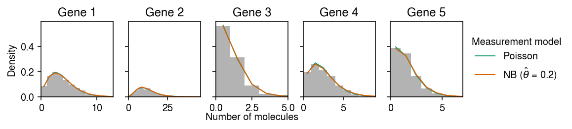
Fit the model to a simulated example, fixing the hyperparameters to the ground truth values. (This only updates the variational approximation.) As a baseline, fit a Gamma expression model to each gene assuming a Poisson measurement model.
x, s, lam, u, log_mean, log_inv_disp, theta = simulate_nb_gamma(n=1000, p=5, theta=0.2, seed=1)
par = np.array([scmodes.ebpm.ebpm_gamma(x[:,j].ravel(), s.ravel()) for j in range(x.shape[1])])
log_mean_hat, log_inv_disp_hat, log_meas_disp_hat, alpha, beta, gamma, delta, elbo = scmodes.ebnbm.ebnbm_gamma(
  x,
  s,
  init=np.hstack([np.exp(log_inv_disp).ravel(), np.exp(-log_mean + log_inv_disp).ravel(), theta]),
  tol=1e-5,
  extrapolate=False,
  fix_g=True,
  fix_theta=True)
Make sure we didn’t mess up the parameterization.
cm = plt.get_cmap('Dark2')
plt.clf()
fig, ax = plt.subplots(1, 5, sharey=True)
fig.set_size_inches(8, 2)

for i, a in enumerate(ax):
  y = np.arange(x[:,i].max() + 1)
  # Poisson measurement => NB observation
  pmf = dict()
  pmf['Poisson'] = st.nbinom(n=np.exp(par[i,1]), p=1 / (1 + (s * np.exp(par[i,0] - par[i,1])))).pmf(y).mean(axis=0)
  # NB measurement => Monte Carlo integral
  n_samples = 1000
  Ghat = st.gamma(a=np.exp(log_inv_disp_hat[:,i]), scale=np.exp(log_mean_hat[:,i] - log_inv_disp_hat[:,i]))
  temp = Ghat.rvs(size=(n_samples, y.shape[0], 1))
  pmf[rf'NB ($\hat\theta$ = {np.exp(log_meas_disp_hat):.2g})'] = st.nbinom(n=np.exp(-log_meas_disp_hat), p=1 / (1 + s[0] * temp * np.exp(log_meas_disp_hat))).pmf(y.reshape(-1, 1)).mean(axis=0)

  ax[i].hist(x[:,i], bins=y, color='0.7', density=True)
  for j, k in enumerate(pmf):
    ax[i].plot(y + .5, pmf[k], c=cm(j), lw=1, label=k)
  ax[i].set_title(f'Gene {i+1}')
  ax[i].set_xlim(0, x[:,i].max())

ax[0].set_ylabel('Density')
ax[-1].legend(title='Measurement model', frameon=False, bbox_to_anchor=(1, .5), loc='center left')
a = fig.add_subplot(111, frameon=False, xticks=[], yticks=[])
a.set_xlabel('Number of molecules', labelpad=16)
fig.tight_layout(pad=0.5)
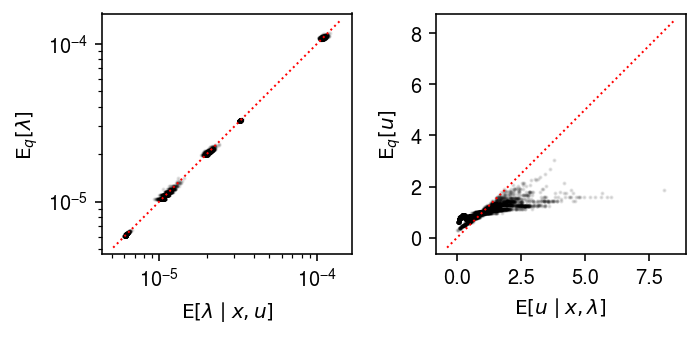
Compare the true posterior against the variational approximation.
plt.clf()
fig, ax = plt.subplots(1, 2)
fig.set_size_inches(5, 2.5)
for a in ax:
  a.set_aspect('equal', adjustable='datalim')

ax[0].set_xscale('log')
ax[0].set_yscale('log')
ax[0].scatter(((x + np.exp(log_inv_disp)) / (s * u + np.exp(log_inv_disp - log_mean))).ravel(), (alpha / beta).ravel(), s=1, c='k', alpha=0.1)
lim = ax[0].get_xlim()
ax[0].plot(lim, lim, lw=1, ls=':', c='r')
ax[0].set_xlabel(r'$\mathrm{E}[\lambda \mid x, u]$')
ax[0].set_ylabel(r'$\mathrm{E}_q[\lambda]$')

ax[1].scatter(((x + theta) / (s * lam + theta)), (gamma / delta).ravel(), s=1, c='k', alpha=0.1)
lim = ax[1].get_xlim()
ax[1].plot(lim, lim, lw=1, ls=':', c='r')
ax[1].set_xlabel(r'$\mathrm{E}[u \mid x, \lambda]$')
ax[1].set_ylabel(r'$\mathrm{E}_q[u]$')

fig.tight_layout()
Now, fit the model initialized at the ground truth hyperparameters, fixing \(\theta\).
fit0 = scmodes.ebnbm.ebnbm_gamma(
  x,
  s,
  init=np.hstack([np.exp(log_inv_disp).ravel(), np.exp(-log_mean + log_inv_disp).ravel(), theta]),
  tol=1e-4,
  max_iters=300_000,
  extrapolate=True,
  fix_g=False,
  fix_theta=True)
fit1 = scmodes.ebnbm.ebnbm_gamma(
  x,
  s,
  init=np.hstack([np.exp(log_inv_disp).ravel(), np.exp(-log_mean + log_inv_disp).ravel(), theta]),
  tol=1e-5,
  max_iters=300_000,
  extrapolate=True,
  fix_g=False,
  fix_theta=True)
with open('/scratch/midway2/aksarkar/modes/ebnbm-sim-ex-1e-5.pkl', 'wb') as f:
  pickle.dump(fit1, f)
with open('/scratch/midway2/aksarkar/modes/ebnbm-sim-ex-1e-5.pkl', 'rb') as f:
  log_mean_hat, log_inv_disp_hat, log_meas_disp_hat, alpha, beta, gamma, delta, elbo = pickle.load(f)
Plot the fitted observation models against the observed data.
cm = plt.get_cmap('Dark2')
plt.clf()
fig, ax = plt.subplots(1, 5, sharey=True)
fig.set_size_inches(8, 2)

for i, a in enumerate(ax):
  y = np.arange(x[:,i].max() + 1)
  # Poisson measurement => NB observation
  pmf = dict()
  pmf['Poisson'] = st.nbinom(n=np.exp(par[i,1]), p=1 / (1 + (s * np.exp(par[i,0] - par[i,1])))).pmf(y).mean(axis=0)
  # NB measurement => Monte Carlo integral
  n_samples = 1000
  Ghat = st.gamma(a=np.exp(log_inv_disp_hat[:,i]), scale=np.exp(log_mean_hat[:,i] - log_inv_disp_hat[:,i]))
  temp = Ghat.rvs(size=(n_samples, y.shape[0], 1))
  pmf[rf'NB ($\hat\theta$ = {np.exp(log_meas_disp_hat):.2g})'] = st.nbinom(n=np.exp(-log_meas_disp_hat), p=1 / (1 + s[0] * temp * np.exp(log_meas_disp_hat))).pmf(y.reshape(-1, 1)).mean(axis=0)

  ax[i].hist(x[:,i], bins=y, color='0.7', density=True)
  for j, k in enumerate(pmf):
    ax[i].plot(y + .5, pmf[k], c=cm(j), lw=1, label=k)
  ax[i].set_title(f'Gene {i+1}')
  ax[i].set_xlim(0, x[:,i].max())

ax[0].set_ylabel('Density')
ax[-1].legend(title='Measurement model', frameon=False, bbox_to_anchor=(1, .5), loc='center left')
a = fig.add_subplot(111, frameon=False, xticks=[], yticks=[])
a.set_xlabel('Number of molecules', labelpad=16)
fig.tight_layout(pad=0.5)
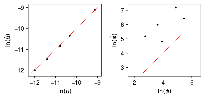
Compare the estimated expression models against the ground truth.
plt.clf()
fig, ax = plt.subplots(1, 2)
fig.set_size_inches(5, 2.5)
for a in ax:
  a.set_aspect('equal', 'datalim')
ax[0].scatter(log_mean, log_mean_hat, s=4, c='k')
lim = ax[0].get_xlim()
ax[0].plot(lim, lim, lw=1, ls=':', c='r')
ax[0].set_xlabel('$\ln(\mu)$')
ax[0].set_ylabel('$\ln(\hat\mu)$')
ax[1].scatter(log_inv_disp, log_inv_disp_hat, s=4, c='k')
lim = ax[1].get_xlim()
ax[1].plot(lim, lim, lw=1, ls=':', c='r')
ax[1].set_xlabel('$\ln(\phi)$')
ax[1].set_ylabel('$\ln(\hat\phi)$')
fig.tight_layout()
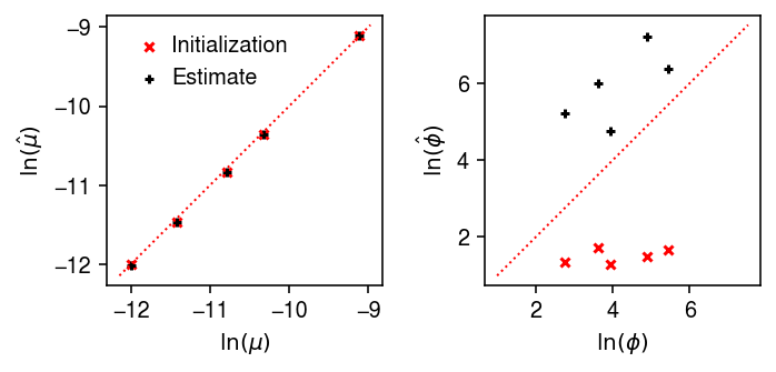
Now fit the model, fixing \(\theta\) to the ground truth, and initializing the expression models at the MLE of a Gamma expression model assuming a Poisson measurement model.
par = np.array([scmodes.ebpm.ebpm_gamma(x[:,j], s.ravel()) for j in range(x.shape[1])])
init = np.hstack([np.exp(par[:,1]), np.exp(par[:,1] - par[:,0]), theta])
fit2 = scmodes.ebnbm.ebnbm_gamma(
  x,
  s,
  init=init,
  tol=1e-5,
  max_iters=300_000,
  extrapolate=True,
  fix_g=False,
  fix_theta=True)
with open('/scratch/midway2/aksarkar/modes/ebnbm-sim-ex-1e-5-pois-init.pkl', 'wb') as f:
  pickle.dump(fit2, f)
with open('/scratch/midway2/aksarkar/modes/ebnbm-sim-ex-1e-5-pois-init.pkl', 'rb') as f:
  log_mean_hat, log_inv_disp_hat, log_meas_disp_hat, alpha, beta, gamma, delta, elbo = pickle.load(f)
Compare the fitted expression models against the ground truth.
plt.clf()
fig, ax = plt.subplots(1, 2)
fig.set_size_inches(5, 2.5)
for a in ax:
  a.set_aspect('equal', 'datalim')
ax[0].scatter(log_mean, par[:,0], s=16, c='r', marker='x', label='Initialization')
ax[0].scatter(log_mean, log_mean_hat, s=16, c='k', marker='+', label='Estimate')
lim = ax[0].get_xlim()
ax[0].plot(lim, lim, lw=1, ls=':', c='r')
ax[0].legend(handletextpad=0, frameon=False)
ax[0].set_xlabel('$\ln(\mu)$')
ax[0].set_ylabel('$\ln(\hat\mu)$')

ax[1].scatter(log_inv_disp, par[:,1], s=16, c='r', marker='x', label='Initialization')
ax[1].scatter(log_inv_disp, log_inv_disp_hat, s=16, c='k', marker='+', label='Estimate')
lim = ax[1].get_ylim()
ax[1].plot(lim, lim, lw=1, ls=':', c='r')
ax[1].set_xlabel('$\ln(\phi)$')
ax[1].set_ylabel('$\ln(\hat\phi)$')
fig.tight_layout()
Compute the ELBO as a function of \(\theta\).
def map_ebnbm_gamma(x, s, grid):
  print('initializing')
  par = np.array([scmodes.ebpm.ebpm_gamma(x[:,j], s.ravel()) for j in range(x.shape[1])])
  # exp(20) is finite and large enough
  par = np.ma.masked_invalid(par).filled(20)
  fits = []
  for theta in grid:
    print(f'fitting theta={theta:.3g}')
    fit = scmodes.ebnbm.ebnbm_gamma(
      x,
      s,
      init=np.hstack([np.exp(par[:,1]), np.exp(par[:,1] - par[:,0]), theta]),
      tol=1e-4,
      max_iters=100_000,
      extrapolate=True,
      fix_g=False,
      fix_theta=True)
    # Warm start
    par = np.vstack(fit[:2]).T
    fits.append(fit)
  return fits
grid = np.logspace(-3, 0, 40)
fits = map_ebnbm_gamma(x, s, grid)
elbo = np.array([f[-1] for f in fits])
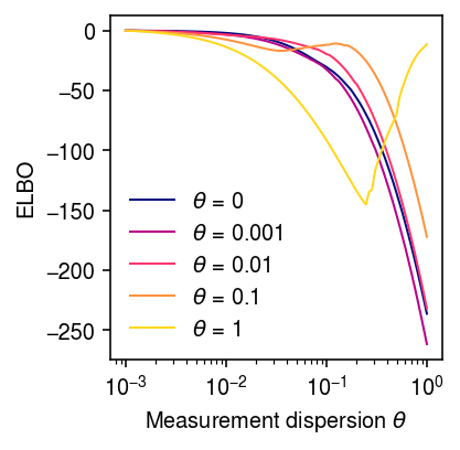
plt.clf()
plt.gcf().set_size_inches(2.5, 2.5)
plt.xscale('log')
plt.plot(grid, elbo, lw=1, c='k')
plt.axvline(x=0.2, lw=1, ls=':', c='r')
plt.xticks(np.logspace(-3, 0, 4))
plt.xlabel(r'Measurement dispersion $\theta$')
plt.ylabel('ELBO')
plt.tight_layout()
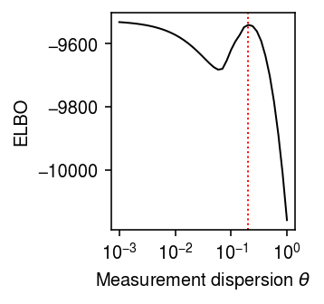
Find the local minimum in the ELBO.
idx = np.where((np.sign(np.diff(elbo)) + 1) / 2)
grid[idx][0], elbo[idx][0]
(0.05878016072274915, -9681.893026800943)
Try running VBEM to stricter tolerance for this choice of \(\theta\).
par = np.array([scmodes.ebpm.ebpm_gamma(x[:,j], s.ravel()) for j in range(x.shape[1])])
init = np.hstack([np.exp(par[:,1]), np.exp(par[:,1] - par[:,0]), grid[idx][0]])
fit3 = scmodes.ebnbm.ebnbm_gamma(
  x,
  s,
  init=init,
  tol=1e-6,
  max_iters=300_000,
  extrapolate=True,
  fix_g=False,
  fix_theta=True)
fit3[-1]
-9681.60485796223
Try initializing VBEM at the ground truth for this choice of \(\theta\).
init = np.hstack([np.exp(log_inv_disp).ravel(), np.exp(-log_mean + log_inv_disp).ravel(), grid[idx][0]])
fit4 = scmodes.ebnbm.ebnbm_gamma(
  x,
  s,
  init=init,
  tol=1e-6,
  max_iters=300_000,
  extrapolate=True,
  fix_g=False,
  fix_theta=True)
fit4[-1]
-9718.192640132213
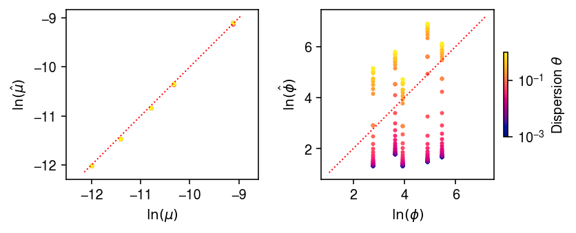
Look at what’s happening for small \(\theta\), by comparing the estimated expression models.
cm = colorcet.cm['bmy']
plt.clf()
fig, ax = plt.subplots(1, 2)
fig.set_size_inches(6, 2.5)
for a in ax:
  a.set_aspect('equal', 'datalim')

for theta, fit in zip(grid, fits):
  c = (np.log(theta) - np.log(1e-3)) / (-np.log(1e-3))
  ax[0].scatter(log_mean, fit[0], s=4, c=np.array(cm(c)).reshape(1, -1))
  ax[1].scatter(log_inv_disp, fit[1], s=4, c=np.array(cm(c)).reshape(1, -1))

lim = ax[0].get_xlim()
ax[0].plot(lim, lim, lw=1, ls=':', c='r')
ax[0].set_xlabel('$\ln(\mu)$')
ax[0].set_ylabel('$\ln(\hat\mu)$')

lim = ax[1].get_ylim()
ax[1].plot(lim, lim, lw=1, ls=':', c='r')
ax[1].set_xlabel('$\ln(\phi)$')
ax[1].set_ylabel('$\ln(\hat\phi)$')

cb = plt.colorbar(matplotlib.cm.ScalarMappable(matplotlib.colors.LogNorm(vmin=1e-3, vmax=1), cmap=cm),
                  fraction=0.05, shrink=0.5)
cb.set_label(r'Dispersion $\theta$')
plt.tight_layout()
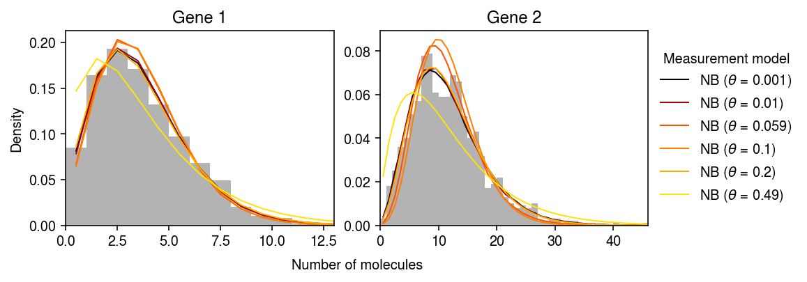
Compare the estimated observation models, focusing on simulated genes 1 and 2.
cm = colorcet.cm['fire']
plt.clf()
fig, ax = plt.subplots(1, 2)
fig.set_size_inches(8, 3)

for i, a in enumerate(ax):
  y = np.arange(x[:,i].max() + 1)
  # NB measurement => Monte Carlo integral
  pmf = dict()
  n_samples = 5000
  query = (0, 13, 23, 26, 30, 35)
  for j in query:
    Ghat = st.gamma(a=np.exp(fits[j][1][:,i]), scale=np.exp(fits[j][0][:,i] - fits[j][1][:,i]))
    temp = Ghat.rvs(size=(n_samples, y.shape[0], 1))
    pmf[rf'NB ($\theta$ = {grid[j]:.2g})'] = st.nbinom(n=1 / grid[j], p=1 / (1 + s[0] * temp * grid[j])).pmf(y.reshape(-1, 1)).mean(axis=0)

  ax[i].hist(x[:,i], bins=y, color='0.7', density=True)
  for j, k in zip(query, pmf):
    z = (np.log(grid[j]) - np.log(1e-3)) / (-np.log(1e-3))
    ax[i].plot(y + .5, pmf[k], c=cm(z), lw=1, label=k)
  ax[i].set_title(f'Gene {i+1}')
  ax[i].set_xlim(0, x[:,i].max())

ax[0].set_ylabel('Density')
ax[-1].legend(title='Measurement model', frameon=False, bbox_to_anchor=(1, .5), loc='center left')
a = fig.add_subplot(111, frameon=False, xticks=[], yticks=[])
a.set_xlabel('Number of molecules', labelpad=24)
fig.tight_layout(pad=0.5)
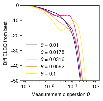
Look at the ELBO as a function of \(\theta\), for data simulated under several different choices of \(\theta\).
elbo = dict()
grid = np.logspace(-3, 0, 100)
for theta0 in (0, 1e-3, 1e-2, 0.1, 1):
  print(f'theta0 = {theta0:.3g}')
  x, s, lam, u, log_mean, log_inv_disp, theta = simulate_nb_gamma(n=100, p=5, theta=theta0, seed=10)
  fits = map_ebnbm_gamma(x, s, grid)
  elbo[theta0] = np.array([f[-1] for f in fits])
cm = colorcet.cm['bmy']
plt.clf()
plt.gcf().set_size_inches(3, 3)
plt.xscale('log')
for i, k in enumerate(elbo):
  if k > 0:
    z = (np.log(k) - np.log(1e-5)) / (1 - np.log(1e-5))
  else:
    z = 0
  plt.plot(grid, elbo[k] - elbo[k].max(), lw=1, c=cm(z), label=rf'$\theta$ = {k:.3g}')
plt.xticks(np.logspace(-3, 0, 4))
plt.legend(frameon=False)
plt.xlabel(r'Measurement dispersion $\theta$')
plt.ylabel('Diff ELBO from best')
plt.tight_layout()
Look more closely at the “phase change” between \(\theta = 0.01\) and \(\theta = 0.1\)
elbo = dict()
grid = np.logspace(-3, 0, 100)
for theta0 in np.logspace(-2, -1, 5):
  print(f'theta0 = {theta0:.3g}')
  x, s, lam, u, log_mean, log_inv_disp, theta = simulate_nb_gamma(n=100, p=5, theta=theta0, seed=10)
  fits = map_ebnbm_gamma(x, s, grid)
  elbo[theta0] = np.array([f[-1] for f in fits])
cm = colorcet.cm['bmy']
plt.clf()
plt.gcf().set_size_inches(3, 3)
plt.xscale('log')
for i, k in enumerate(elbo):
  z = (np.log(k) - np.log(1e-2)) / (np.log(.1) - np.log(1e-2))
  plt.plot(grid, elbo[k] - elbo[k].max(), lw=1, c=cm(z), label=rf'$\theta$ = {k:.3g}')
plt.xticks(np.logspace(-3, 0, 4))
plt.legend(frameon=False)
plt.xlabel(r'Measurement dispersion $\theta$')
plt.ylabel('Diff ELBO from best')
plt.ylim(-50, 0)
plt.tight_layout()
Moment-matching approximation
Consider gene \(j\), and assume \(a = \phi^{-1}\), \(b = \mu^{-1}\phi^{-1}\). Then,
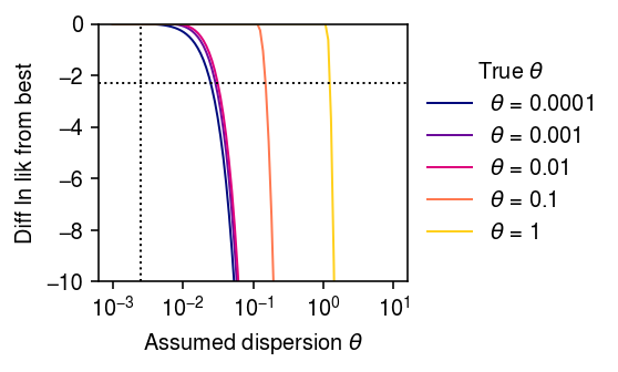
\begin{align} \E{\lambda_i} &= \mu\\ \V[\lambda_i] &= \mu^2\phi\\ \E{x_i} &= \E{\E{x_i \mid s_i, \lambda_i}} = s_i \mu\\ \V[x_i] &= \E{\V[x_i \mid s_i, \lambda_i]} + \V[\E{x_i \mid s_i \lambda_i}]\\ &= \E{s_i \lambda_i + (s_i \lambda_i)^2 \theta} + \V[s_i \lambda_i]\\ &= s_i \mu + s_i^2 \mu^2 (\phi + \theta + \phi\theta) \end{align}This result suggests an approximate approach to characterize the profile likelihood of the data with respect to \(\theta\), that uses an NB model with dispersion \(d = \phi + \theta + \phi\theta\). As a proof of concept, fit the model using the Nelder-Mead algorithm.
def _loss(par, x, s, theta0):
  mu, phi = np.exp(par)
  theta = phi + theta0 + phi * theta0
  return -st.nbinom(n=1 / theta, p=1 / (1 + s * mu * theta)).logpmf(x).mean()

np.random.seed(1)
s = 1e5
n = 100

log_mu = -10
log_phi = -6
lam = st.gamma(a=np.exp(-log_phi), scale=np.exp(log_mu + log_phi)).rvs(n)

fits = dict()
grid = np.logspace(-3, 1, 100)
for theta0 in np.logspace(-4, 0, 5):
  print(f'fitting theta0 = {theta0:.1g}')
  u = st.gamma(a=1 / theta0, scale=theta0).rvs(n)
  x = st.poisson(s * lam * u).rvs(n)
  fits[theta0] = [so.minimize(_loss, x0=[log_mu, log_phi], args=(x, s, theta), method='Nelder-Mead')
                  for theta in grid]
cm = colorcet.cm['bmy']
plt.clf()
plt.gcf().set_size_inches(4, 2.5)
plt.xscale('log')
for i, k in enumerate(fits):
  temp = n * np.array([-f.fun for f in fits[k]])
  temp -= temp.max()
  c = (np.log(k) - np.log(1e-4)) / (1 - np.log(1e-4))
  plt.plot(grid, temp, lw=1, c=cm(c), label=rf'$\theta$ = {k:.1g}')
plt.axvline(x=np.exp(log_phi), lw=1, ls=':', c='k')
plt.axhline(y=-np.log(10), lw=1, ls=':', c='k')
plt.legend(title=r'True $\theta$', frameon=False, loc='center left', bbox_to_anchor=(1, .5))
plt.xticks(np.logspace(-3, 1, 5))
plt.ylim(-10, 0)
plt.xlabel(r'Assumed dispersion $\theta$')
plt.ylabel('Diff ln lik from best')
plt.tight_layout()
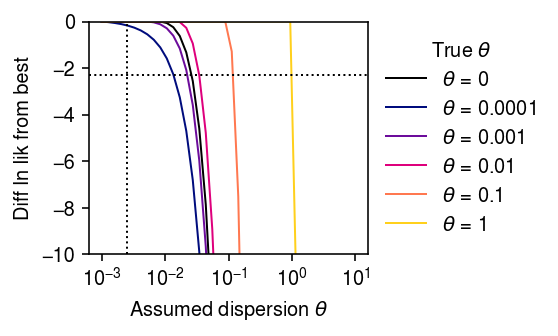
Now, fit the model in stages:
- Fit the NB model via unconstrained optimization, yielding MLE \(\hat\mu, \hat{d}\)
- If \(\hat\phi = (\hat{d} - \theta) / (1 + \theta) < 0\), then fit the NB model, fixing dispersion \(\theta\).
def _fit_one(x, s, theta, tol=1e-7):
  fit = scmodes.ebpm.wrappers.ebpm_gamma(x, s, tol=tol)
  if (np.exp(-fit[1]) - theta) / (1 + theta) < 0:
    fit = scmodes.ebpm.wrappers.ebpm_gamma(x, s, a=1 / theta, tol=tol)
  return fit

def _fit(x, s, grid):
  return np.array([_fit_one(x, s, theta) for theta in grid])

s = 1e5
n = 1600
log_mu = -10
log_phi = -6

np.random.seed(9)
lam = st.gamma(a=np.exp(-log_phi), scale=np.exp(log_mu + log_phi)).rvs(n)
x = st.poisson(s * lam).rvs(n)

fits = dict()
grid = np.logspace(-3, 1, 40)

print(f'fitting theta0 = 0')
fits[0] = _fit(x, s, grid)
for i, theta0 in enumerate(np.logspace(-4, 0, 5)):
  print(f'fitting theta0 = {theta0:.1g}')
  np.random.seed(i)
  u = st.gamma(a=1 / theta0, scale=theta0).rvs(n)
  x = st.poisson(s * lam * u).rvs(n)
  fits[theta0] = _fit(x, s, grid)
cm = colorcet.cm['bmy']
plt.clf()
plt.gcf().set_size_inches(4, 2.5)
plt.xscale('log')
for i, k in enumerate(fits):
  temp = fits[k][:,-1] - fits[k][:,-1].max()
  if k > 0:
    c = cm((np.log(k) - np.log(1e-4)) / (1 - np.log(1e-4)))
  else:
    c = 'k'
  plt.plot(grid, temp, lw=1, c=c, label=rf'$\theta$ = {k:.1g}')
plt.axvline(x=np.exp(log_phi), lw=1, ls=':', c='k')
plt.axhline(y=-np.log(10), lw=1, ls=':', c='k')
plt.legend(title=r'True $\theta$', frameon=False, loc='center left', bbox_to_anchor=(1, .5))
plt.xticks(np.logspace(-3, 1, 5))
plt.ylim(-10, 0)
plt.xlabel(r'Assumed dispersion $\theta$')
plt.ylabel('Diff ln lik from best')
plt.tight_layout()
Application to control data
Fit the EBNBM model to each control data set.
def _init(j, x, s):
  return scmodes.ebpm.ebpm_gamma(x[:,j].ravel(), s.ravel())

def _fit(theta, x, s, par):
  return scmodes.ebnbm.ebnbm_gamma(
    x,
    s,
    init=np.hstack([np.exp(par[:,1]), np.exp(par[:,1] - par[:,0]), theta]),
    tol=1e-3,
    max_iters=100_000,
    extrapolate=True,
    fix_g=False,
    fix_theta=True)

tasks = control
d = tasks[int(os.environ['SLURM_ARRAY_TASK_ID'])]
with mp.Pool() as pool:
  dat = data[d]()
  x = dat.X.A
  s = x.sum(axis=1, keepdims=True)
  par = pool.map(ft.partial(_init, x=x, s=s), range(x.shape[1]))
  # Important: ebpm_gamma can return np.inf is data is consistent with Poisson
  # observation model. exp(20) is finite and large enough.
  par = np.ma.masked_invalid(np.array(par)).filled(20)
  grid = np.logspace(-3, 1, 20)
  fits = pool.map(ft.partial(_fit, x=x, s=s, par=par), grid)
with open(f'/scratch/midway2/aksarkar/modes/ebnbm/ebnbm-{d}.pkl', 'wb') as f:
  pickle.dump(dict(zip(grid, fits)), f)
sbatch --partition=gpu2 --gres=gpu:1 -w midway2-gpu05 -n1 -c28 --exclusive -a 4
#!/bin/bash
source activate scmodes
python <<EOF
<<imports>>
import multiprocessing as mp
import pickle
import os
<<data>>
<<fit>>
EOF
Read the fitted models.
elbo = dict()
for k in data:
  if k in control:
    with open(f'/scratch/midway2/aksarkar/modes/ebnbm/ebnbm-{k}.pkl', 'rb') as f:
      fits = pickle.load(f)
      elbo[k] = pd.Series({theta: fits[theta][-1] for theta in fits})
elbo = pd.DataFrame(elbo)
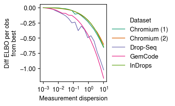
labels = ['Chromium (1)', 'Chromium (2)', 'Drop-Seq', 'GemCode', 'InDrops']
keys = ['chromium1', 'chromium2', 'dropseq', 'gemcode', 'indrops']
cm = plt.get_cmap('Dark2')
plt.clf()
plt.gcf().set_size_inches(4, 2.5)
plt.xscale('log')
for i, (k, l) in enumerate(zip(keys, labels)):
  n, p = data[k]().shape
  diff = elbo[k] - elbo[k].max()
  plt.plot(elbo.index, diff / (n * p), lw=1, label=l, c=cm(i))
plt.legend(title='Dataset', frameon=False, loc='center left', bbox_to_anchor=(1, .5))
plt.xticks(np.logspace(-3, 1, 5))
plt.xlabel(r'Measurement dispersion')
plt.ylabel('Diff ELBO per obs\nfrom best')
plt.tight_layout()
Fit the heuristic to each data set.
def _fit_one(x, s, theta, tol=1e-7):
  fit = scmodes.ebpm.wrappers.ebpm_gamma(x, s, tol=tol)
  if (np.exp(-fit[1]) - theta) / (1 + theta) < 0:
    fit = scmodes.ebpm.wrappers.ebpm_gamma(x, s, a=1 / theta, tol=tol)
  return fit

tasks = control
d = tasks[int(os.environ['SLURM_ARRAY_TASK_ID'])]
with mp.Pool() as pool:
  dat = data[d]()
  x = dat.X.A
  s = x.sum(axis=1)
  fits = []
  for theta in np.logspace(-3, -2, 100):
    _fit = ft.partial(_fit_one, s=s, theta=theta)
    fits.append(pool.map(_fit, x.T))
  fits = np.stack(fits)
  np.save(f'/scratch/midway2/aksarkar/modes/ebnbm/nb-heuristic-{d}.npy', fits)
sbatch --partition=broadwl -n1 -c28 --exclusive -a 0-4
#!/bin/bash
source activate scmodes
python <<EOF
<<imports>>
import multiprocessing as mp
import os
<<data>>
<<fit-heuristic>>
EOF
Copy the fitted models to permanent storage.
rsync -au /scratch/midway2/aksarkar/modes/ebnbm/ /project2/mstephens/aksarkar/projects/singlecell-modes/data/ebnbm/
Read the fitted models.
fits = dict()
for k in control:
  fits[k] = np.load(f'/scratch/midway2/aksarkar/modes/ebnbm/nb-heuristic-{k}.npy')
Plot the profile likelihood.
labels = ['Chromium (1)', 'Chromium (2)', 'Drop-Seq', 'GemCode', 'InDrops']
keys = ['chromium1', 'chromium2', 'dropseq', 'gemcode', 'indrops']

cm = plt.get_cmap('Dark2')
plt.clf()
plt.gcf().set_size_inches(4, 2.5)
plt.xscale('log')
grid = np.logspace(-3, -2, 100)
for i, (k, l) in enumerate(zip(keys, labels)):
  temp = fits[k][:,:,-1].sum(axis=1)
  diff = temp - temp.max()
  plt.plot(grid, diff, lw=1, label=l, c=cm(i))
plt.ylim(-20, 0)
plt.axhline(y=-np.log(10), lw=1, ls=':', c='k')
plt.legend(title='Dataset', frameon=False, loc='center left', bbox_to_anchor=(1, .5))
plt.xlabel(r'Assumed dispersion')
plt.ylabel('Difference in ln likelihood\nfrom best')
plt.tight_layout()
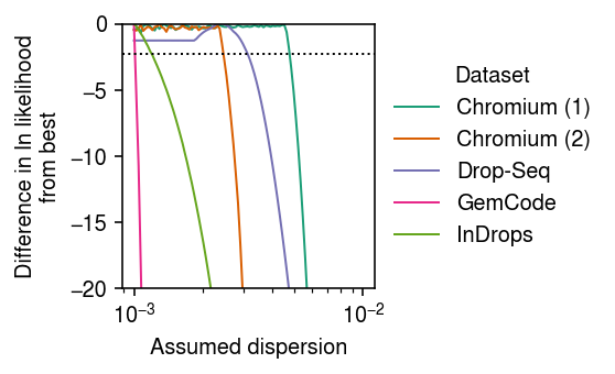
Report the smallest \(\theta\) for which the likelihood ratio is \(< 1/10\) compared to the best \(\theta\).
thresh = -np.log(10)
grid = np.logspace(-3, -2, 100)
thetahat = dict()
for k in keys:
  l = fits[k][:,:,-1].sum(axis=1)
  l -= l.max()
  thetahat[k] = grid[np.where(l < thresh)[0][0]]
pd.Series(thetahat)
chromium1    0.004863
chromium2    0.002477
dropseq      0.003199
gemcode      0.001024
indrops      0.001205
dtype: float64
Compare the bound on the measurement dispersion \(\theta\) to the level of total dispersion estimated in highly expressed genes in control data.
count_thresh = 10
dhat = dict()
for k in keys:
  dat = data[k]()
  x = dat.X.A
  s = x.sum(axis=1)
  x = x[:,x.mean(axis=0) > count_thresh]
  temp = [scmodes.ebpm.ebpm_gamma(x[:,j], s) for j in range(x.shape[1])]
  if temp:
    dhat[k] = pd.DataFrame(np.array(temp), columns=['log_mean', 'log_inv_disp', 'llik'])
dhat = pd.concat(dhat)
(dhat
 ['log_inv_disp']
 .apply(lambda x: np.exp(-x))
 .groupby(level=0)
 .agg([np.mean, np.std, np.median]))
mean       std    median
chromium1  0.018258  0.013050  0.016499
chromium2  0.021233  0.014184  0.022940
dropseq    0.391793  0.567800  0.104669
gemcode    0.031384  0.032980  0.017520
indrops    0.003968  0.006656  0.000000
Comparing measurement dispersion to biological variability
Fit an NB observation model to highly expressed genes (mean molecule count > 10) in biological data sets.
thresh = 10

def _fit_one(j, x, s):
  return scmodes.ebpm.ebpm_gamma(x[:,j].A.ravel(), s)

tasks = non_control
d = tasks[int(os.environ['SLURM_ARRAY_TASK_ID'])]
with mp.Pool() as pool:
  dat = data[d]()
  s = dat.X.sum(axis=1).A.ravel()
  x = dat[:,dat.X.mean(axis=0) > thresh].X
  _fit = ft.partial(_fit_one, x=x, s=s)
  fits = pool.map(_fit, range(x.shape[1]))
  fits = np.array(fits)
  np.save(f'/scratch/midway2/aksarkar/modes/ebnbm/nb-obs-{d}.npy', fits)
sbatch --partition=broadwl -n1 -c28 --exclusive -a 1-10
#!/bin/bash
source activate scmodes
python <<EOF
<<imports>>
import multiprocessing as mp
import os
<<data>>
<<fit-pois-gamma>>
EOF
Read the fitted models.
fits = dict()
for k in non_control:
  f = np.load(f'/scratch/midway2/aksarkar/modes/ebnbm/nb-obs-{k}.npy')
  fits[k] = pd.DataFrame(f, columns=['log_mean', 'log_inv_disp', 'llik'])
fits = pd.concat(fits)
Look at the distribution of estimated dispersions.
(fits['log_inv_disp']
 .apply(lambda x: np.exp(-x))
 .groupby(level=0)
 .agg([np.median, np.mean, np.std]))
median      mean       std
b_cells              0.020502  0.021608  0.023738
brain                1.509569  1.509569  0.744572
cytotoxic_t          0.020181  0.027366  0.026903
cytotoxic_t-b_cells  0.024305  0.111044  0.474656
cytotoxic_t-naive_t  0.023493  0.031068  0.027497
ipsc                 0.054512  0.074847  0.134037
kidney               0.115725  0.266653  0.387907
liver-caudate-lobe   0.114579  0.138094  0.145873
pbmc_10k_v3          0.237059  0.596076  1.495602
retina               1.698007  2.088869  1.676650