Distribution deconvolution examples

Introduction
Setup
Results

Introduction

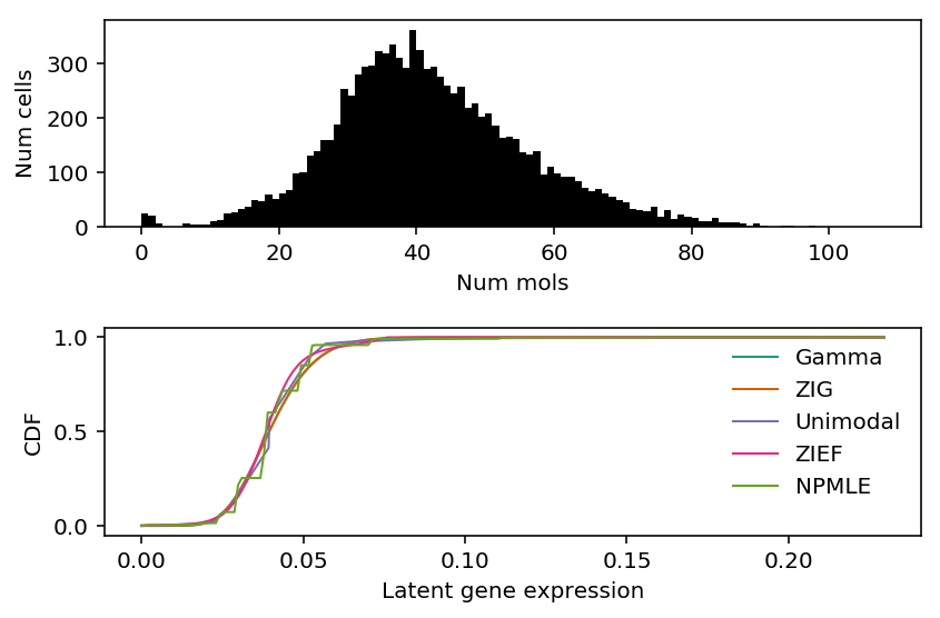
We systematically compared different deconvolution methods on their ability to generalize to held out data. Here, we look at the data and fitted distributions for specific examples.

Setup

import functools as ft
import multiprocessing as mp
import numpy as np
import pandas as pd
import scanpy
import scipy.stats as st
import scipy.special as sp
import scmodes
import sklearn.model_selection as skms

import rpy2.robjects.packages
import rpy2.robjects.pandas2ri
import rpy2.robjects.numpy2ri

rpy2.robjects.pandas2ri.activate()
rpy2.robjects.numpy2ri.activate()

ashr = rpy2.robjects.packages.importr('ashr')
descend = rpy2.robjects.packages.importr('descend')

%matplotlib inline
%config InlineBackend.figure_formats = set(['retina'])

import colorcet
import matplotlib.pyplot as plt
plt.rcParams['figure.facecolor'] = 'w'
plt.rcParams['font.family'] = 'Nimbus Sans'

Results

Test

b_cells = scmodes.dataset.read_10x('/project2/mstephens/aksarkar/projects/singlecell-ideas/data/10xgenomics/b_cells/filtered_matrices_mex/hg19/', return_df=True)
llik_diff = benchmark['b_cells']['npmle'] - benchmark['b_cells']['gamma']
query = llik_diff[llik_diff > 0].sort_values(ascending=False).head(n=1).index

x = b_cells[query].values.ravel()
s = b_cells.sum(axis=1).values.ravel()

plt.clf()
fig, ax = plt.subplots(2, 1)
fig.set_size_inches(6, 4)
ax[0].hist(x, bins=np.arange(x.max() + 1), color='k')
ax[0].set_xlabel('Num mols')
ax[0].set_ylabel('Num cells')

for c, k in zip(plt.get_cmap('Dark2').colors, ['Gamma', 'ZIG', 'Unimodal', 'ZIEF', 'NPMLE']):
  ax[1].plot(*getattr(scmodes.deconvolve, f'fit_{k.lower()}')(x, s), color=c, lw=1, label=k)
ax[1].set_xlabel('Latent gene expression')
ax[1].set_ylabel('CDF')
ax[1].legend(frameon=False)
fig.tight_layout()

Metadata

Read gene metadata.

gene_info = pd.read_csv('/project2/mstephens/aksarkar/projects/singlecell-qtl/data/scqtl-genes.txt.gz', sep='\t', index_col=0)

Spike-in data

Read the results.

benchmark = {
  k: g.reset_index(level=0, drop=True) for k, g in
  (pd.read_csv('/project2/mstephens/aksarkar/projects/singlecell-modes/data/deconv-generalization/control-kl.txt.gz',
               sep='\t', index_col=[0, 1])
   .groupby(level=0))}

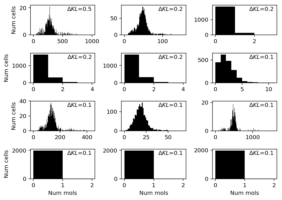
We are primarily interested in cases where NPMLE does better than unimodal, because these could potentially be cases where zeros drive the difference in generalization performance.

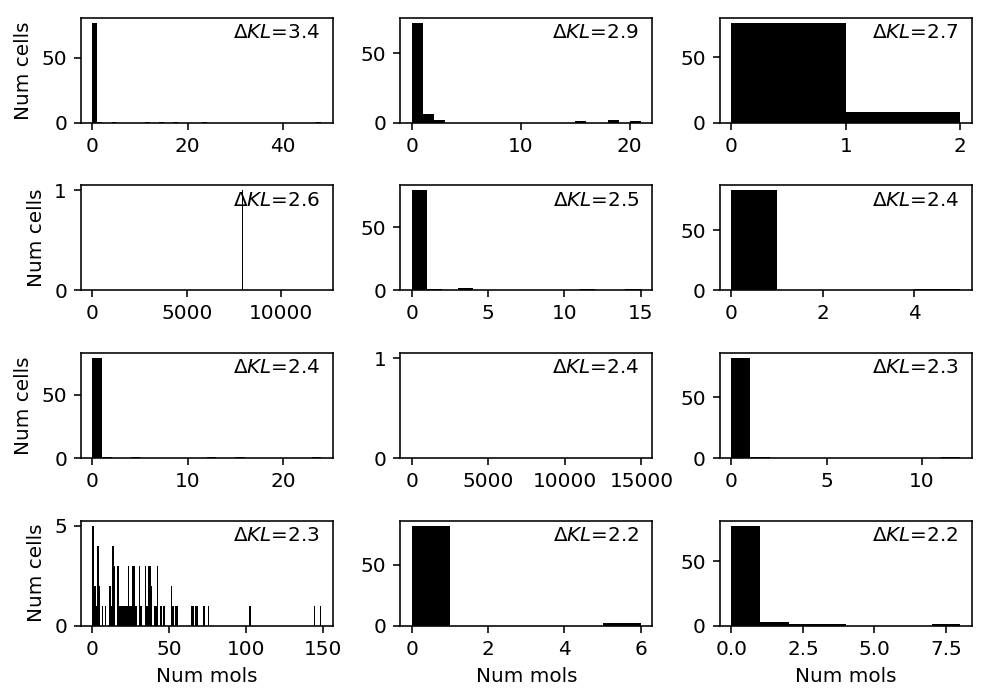
chromium1 = data['chromium1']()
llik_diff = benchmark['chromium1']['npmle'] - benchmark['chromium1']['unimodal']
query = llik_diff[np.logical_and(chromium1.sum(axis=0) > 0, llik_diff > 0)].sort_values(ascending=False).head(n=12).index
plt.clf()
fig, ax = plt.subplots(4, 3)
fig.set_size_inches(7, 5)
for a, k in zip(ax.ravel(), query):
  a.hist(chromium1[:,k], bins=np.arange(chromium1[:,k].max() + 2), color='k')
  a.text(x=.95, y=.95,
         s=f"$\Delta KL$={llik_diff.loc[k]:.1f}",
         horizontalalignment='right',
         verticalalignment='top',
         transform=a.transAxes)
for y in range(ax.shape[0]):
  ax[y][0].set_ylabel('Num cells')
for x in range(ax.shape[1]):
  ax[-1][x].set_xlabel('Num mols')
fig.tight_layout()

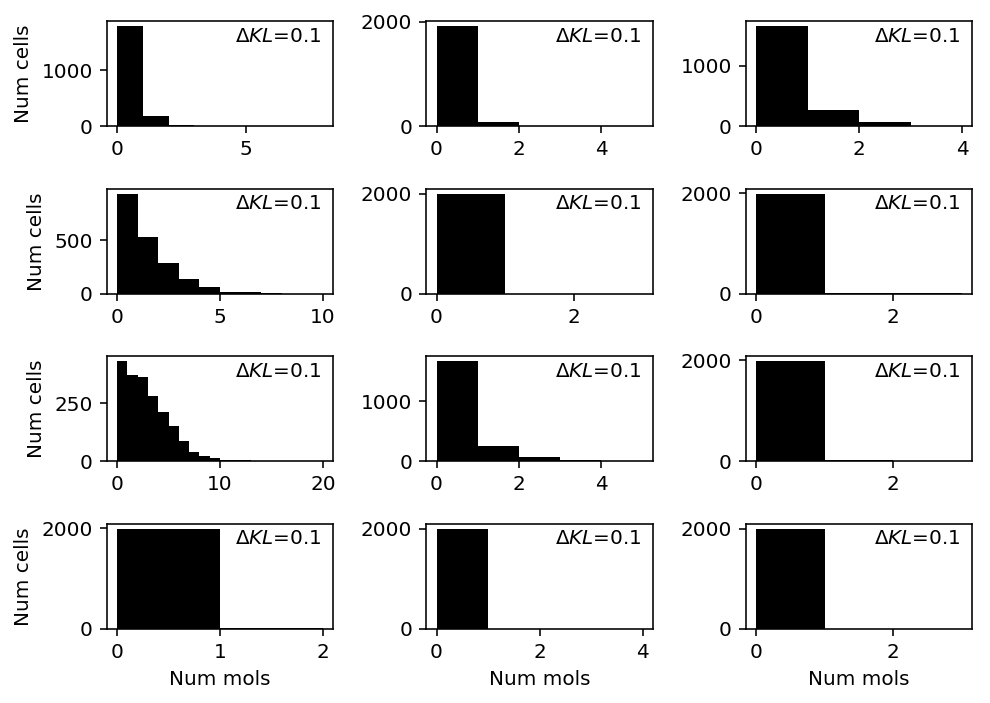
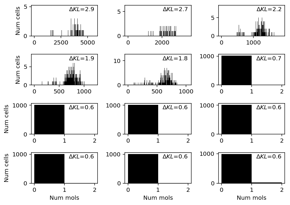
chromium2 = data['chromium2']()
llik_diff = benchmark['chromium2']['npmle'] - benchmark['chromium2']['unimodal']
query = llik_diff[np.logical_and(chromium2.sum(axis=0) > 0, llik_diff > 0)].sort_values(ascending=False).head(n=12).index

plt.clf()
fig, ax = plt.subplots(4, 3)
fig.set_size_inches(7, 5)
for a, k in zip(ax.ravel(), query):
  a.hist(chromium2[:,k], bins=np.arange(chromium2[:,k].max() + 2), color='k')
  a.text(x=.95, y=.95,
         s=f"$\Delta KL$={llik_diff.loc[k]:.1f}",
         horizontalalignment='right',
         verticalalignment='top',
         transform=a.transAxes)
for y in range(ax.shape[0]):
  ax[y][0].set_ylabel('Num cells')
for x in range(ax.shape[1]):
  ax[-1][x].set_xlabel('Num mols')
fig.tight_layout()

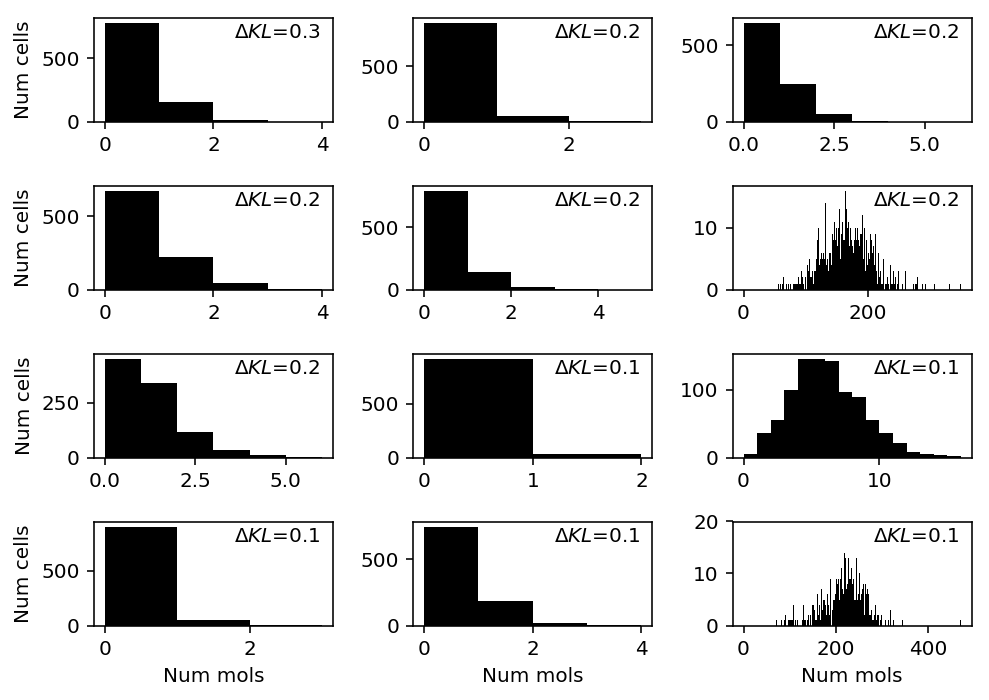
dropseq = data['dropseq']()
llik_diff = benchmark['dropseq']['npmle'] - benchmark['dropseq']['unimodal']
query = benchmark['dropseq'].loc[llik_diff[llik_diff > 0].sort_values(ascending=False).head(n=12).index].index
plt.clf()
fig, ax = plt.subplots(4, 3)
fig.set_size_inches(7, 5)
for a, k in zip(ax.ravel(), query):
  a.hist(dropseq[:,k], bins=np.arange(dropseq[:,k].max() + 2), color='k')
  a.text(x=.95, y=.95,
         s=f"$\Delta KL$={llik_diff.loc[k]:.1f}",
         horizontalalignment='right',
         verticalalignment='top',
         transform=a.transAxes)
for y in range(ax.shape[0]):
  ax[y][0].set_ylabel('Num cells')
for x in range(ax.shape[1]):
  ax[-1][x].set_xlabel('Num mols')
fig.tight_layout()

gemcode = data['gemcode']()
llik_diff = benchmark['gemcode']['npmle'] - benchmark['gemcode']['unimodal']
query = llik_diff[np.logical_and(gemcode.sum(axis=0) > 0, llik_diff > 0)].sort_values(ascending=False).head(n=12).index
plt.clf()
fig, ax = plt.subplots(4, 3)
fig.set_size_inches(7, 5)
for a, k in zip(ax.ravel(), query):
  a.hist(gemcode[:,k], bins=np.arange(gemcode[:,k].max() + 2), color='k')
  a.text(x=.95, y=.95,
         s=f"$\Delta KL$={llik_diff.loc[k]:.1f}",
         horizontalalignment='right',
         verticalalignment='top',
         transform=a.transAxes)
for y in range(ax.shape[0]):
  ax[y][0].set_ylabel('Num cells')
for x in range(ax.shape[1]):
  ax[-1][x].set_xlabel('Num mols')
fig.tight_layout()

indrops = data['indrops']()
llik_diff = benchmark['indrops']['npmle'] - benchmark['indrops']['unimodal']
query = llik_diff[np.logical_and(indrops.sum(axis=0) > 0, llik_diff > 0)].sort_values(ascending=False).head(n=12).index
plt.clf()
fig, ax = plt.subplots(4, 3)
fig.set_size_inches(7, 5)
for a, k in zip(ax.ravel(), query):
  a.hist(indrops[:,k], bins=np.arange(indrops[:,k].max() + 2), color='k')
  a.text(x=.95, y=.95,
         s=f"$\Delta KL$={llik_diff.loc[k]:.1f}",
         horizontalalignment='right',
         verticalalignment='top',
         transform=a.transAxes)
for y in range(ax.shape[0]):
  ax[y][0].set_ylabel('Num cells')
for x in range(ax.shape[1]):
  ax[-1][x].set_xlabel('Num mols')
fig.tight_layout()

Homogeneous populations

Read the results.

benchmark = {
  k: g.reset_index(level=0, drop=True) for k, g in
  (pd.read_csv('/project2/mstephens/aksarkar/projects/singlecell-modes/data/deconv-generalization/homogeneous-kl.txt.gz',
               sep='\t', index_col=[0, 1])
   .groupby(level=0))}

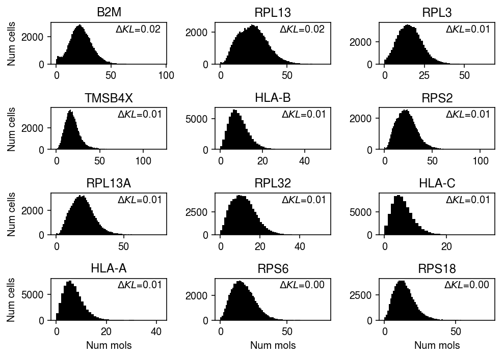
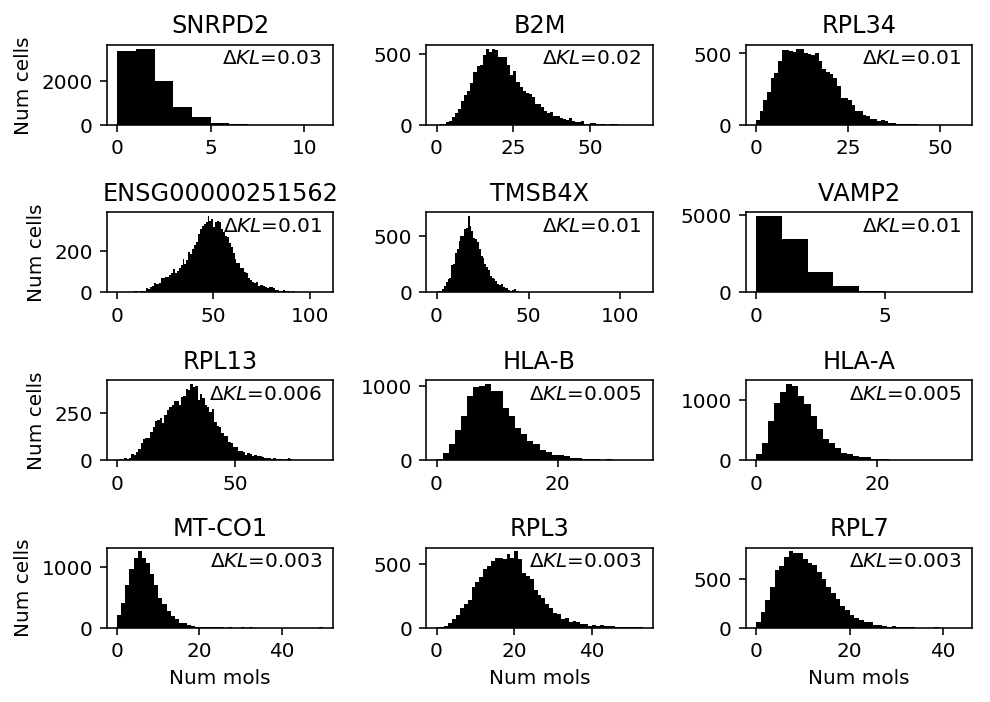
Focus on cases where NPMLE does better than unimodal. Look at B cells.

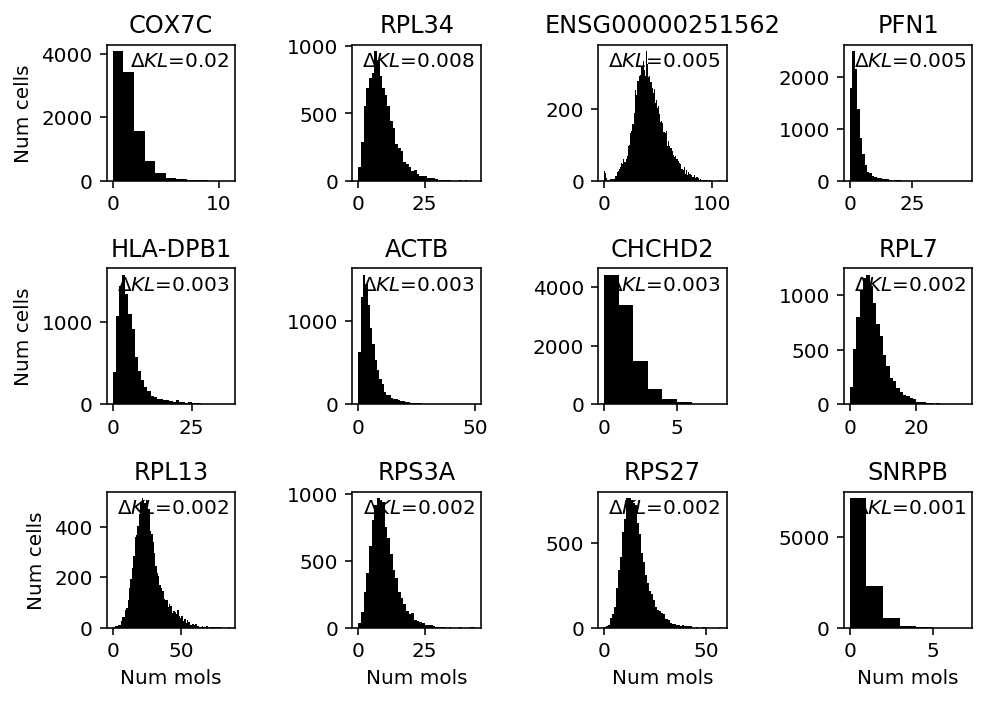
b_cells = scmodes.dataset.read_10x('/project2/mstephens/aksarkar/projects/singlecell-ideas/data/10xgenomics/b_cells/filtered_matrices_mex/hg19/', return_df=True)
llik_diff = benchmark['b_cells']['npmle'] - benchmark['b_cells']['unimodal']
query = llik_diff[llik_diff > 0].sort_values(ascending=False).head(n=12).index

plt.clf()
fig, ax = plt.subplots(3, 4)
fig.set_size_inches(7, 5)
for a, k in zip(ax.ravel(), query):
  a.hist(b_cells.loc[:,k], bins=np.arange(b_cells.loc[:,k].max() + 1), color='k')
  a.text(x=.95, y=.95,
         s=f"$\Delta KL$={llik_diff.loc[k]:.1g}",
         horizontalalignment='right',
         verticalalignment='top',
         transform=a.transAxes)
  a.set_title(gene_info.loc[k, 'name'] if k in gene_info.index else k)
for y in range(ax.shape[0]):
  ax[y][0].set_ylabel('Num cells')
for x in range(ax.shape[1]):
  ax[-1][x].set_xlabel('Num mols')
fig.tight_layout()

Look at cytotoxic T cells.

cytotoxic_t = scmodes.dataset.read_10x('/project2/mstephens/aksarkar/projects/singlecell-ideas/data/10xgenomics/cytotoxic_t/filtered_matrices_mex/hg19/', return_df=True)
llik_diff = benchmark['cytotoxic_t']['npmle'] - benchmark['cytotoxic_t']['unimodal']
query = llik_diff[llik_diff > 0].sort_values(ascending=False).head(n=12).index

plt.clf()
fig, ax = plt.subplots(4, 3)
fig.set_size_inches(7, 5)
for a, k in zip(ax.ravel(), query):
  a.hist(cytotoxic_t.loc[:,k], bins=np.arange(cytotoxic_t.loc[:,k].max() + 1), color='k')
  a.text(x=.95, y=.95,
         s=f"$\Delta KL$={llik_diff.loc[k]:.1g}",
         horizontalalignment='right',
         verticalalignment='top',
         transform=a.transAxes)
  a.set_title(gene_info.loc[k, 'name'] if k in gene_info.index else k)
for y in range(ax.shape[0]):
  ax[y][0].set_ylabel('Num cells')
for x in range(ax.shape[1]):
  ax[-1][x].set_xlabel('Num mols')
fig.tight_layout()

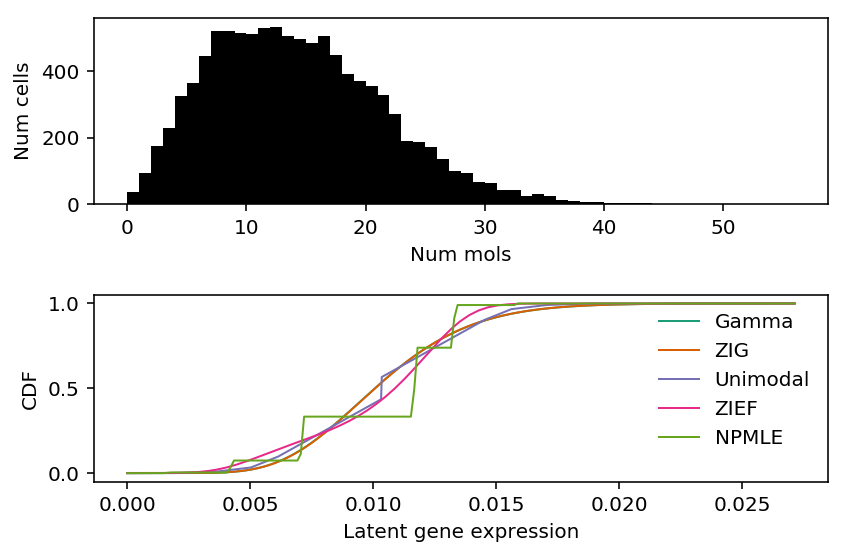
Make sure our choice of discretization for unimodal is acceptable on RPL34.

k = 'ENSG00000109475'
x = cytotoxic_t.loc[:,k]
s = cytotoxic_t.sum(axis=1)

plt.clf()
fig, ax = plt.subplots(2, 1)
fig.set_size_inches(6, 4)
ax[0].hist(x, bins=np.arange(x.max() + 1), color='k')
ax[0].set_xlabel('Num mols')
ax[0].set_ylabel('Num cells')

for c, k in zip(plt.get_cmap('Dark2').colors, ['Gamma', 'ZIG', 'Unimodal', 'ZIEF', 'NPMLE']):
  ax[1].plot(*getattr(scmodes.deconvolve, f'fit_{k.lower()}')(x, s), color=c, lw=1, label=k)
ax[1].set_xlabel('Latent gene expression')
ax[1].set_ylabel('CDF')
ax[1].legend(frameon=False)
fig.tight_layout()

Mengyin Lu previously reported CCL5 could possibly have bimodal expression. Look at the fitted distributions for CCL5.

k = 'ENSG00000161570'
x = cytotoxic_t.loc[:,k]
s = cytotoxic_t.sum(axis=1)

plt.clf()
fig, ax = plt.subplots(2, 1)
fig.set_size_inches(6, 4)
ax[0].hist(x, bins=np.arange(x.max() + 1), color='k')
ax[0].set_xlabel('Num mols')
ax[0].set_ylabel('Num cells')

for c, k in zip(plt.get_cmap('Dark2').colors, ['Gamma', 'ZIG', 'Unimodal', 'ZIEF', 'NPMLE']):
  ax[1].plot(*getattr(scmodes.deconvolve, f'fit_{k.lower()}')(x, s), color=c, lw=1, label=k)
ax[1].set_xlabel('Latent gene expression')
ax[1].set_ylabel('CDF')
ax[1].legend(frameon=False)
fig.tight_layout()

Look at iPSCs.

ipsc_counts = scmodes.dataset.ipsc('/project2/mstephens/aksarkar/projects/singlecell-qtl/data/', n=100, return_df=True)
llik_diff = benchmark['ipsc']['npmle'] - benchmark['ipsc']['unimodal']
query = llik_diff[llik_diff > 0].sort_values(ascending=False).head(n=12).index

plt.clf()
fig, ax = plt.subplots(4, 3)
fig.set_size_inches(7, 5)
for a, k in zip(ax.ravel(), query):
  h = a.hist(ipsc_counts.loc[:,k], bins=np.arange(ipsc_counts.loc[:,k].max() + 1), color='k')
  a.text(x=.95, y=.95,
         s=f"$\Delta KL$={llik_diff.loc[k]:.1g}",
         horizontalalignment='right',
         verticalalignment='top',
         transform=a.transAxes)
  a.set_title(gene_info.loc[k, 'name'])
for y in range(ax.shape[0]):
  ax[y][0].set_ylabel('Num cells')
for x in range(ax.shape[1]):
  ax[-1][x].set_xlabel('Num mols')
fig.tight_layout()

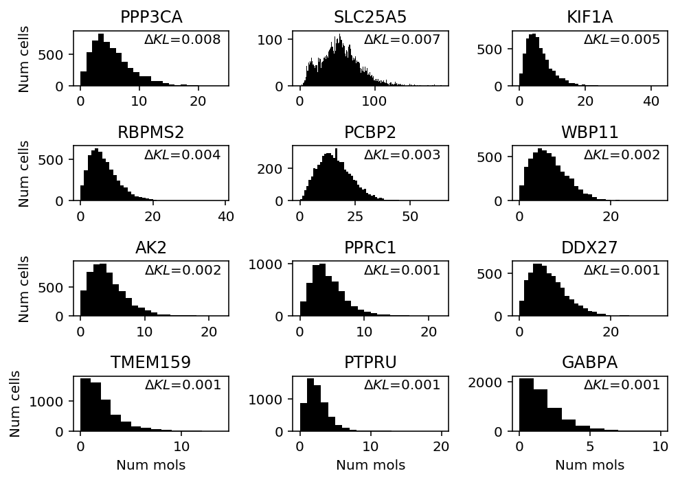
Compare against Gamma.

llik_diff = benchmark['ipsc']['npmle'] - benchmark['ipsc']['gamma']
query = llik_diff[llik_diff > 0].sort_values(ascending=False).head(n=12).index
plt.clf()
fig, ax = plt.subplots(4, 3)
fig.set_size_inches(7, 5)
for a, k in zip(ax.ravel(), query):
  a.hist(ipsc_counts.loc[:,k], bins=np.arange(ipsc_counts.loc[:,k].max() + 1), color='k')
  a.text(x=.95, y=.95,
         s=f"$\Delta KL$={llik_diff.loc[k]:.1g}",
         horizontalalignment='right',
         verticalalignment='top',
         transform=a.transAxes)
  a.set_title(gene_info.loc[k, 'name'])
for y in range(ax.shape[0]):
  ax[y][0].set_ylabel('Num cells')
for x in range(ax.shape[1]):
  ax[-1][x].set_xlabel('Num mols')
fig.tight_layout()

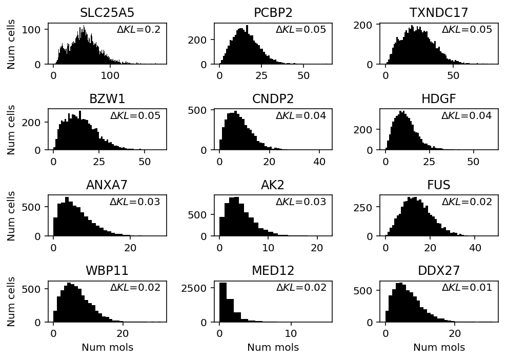
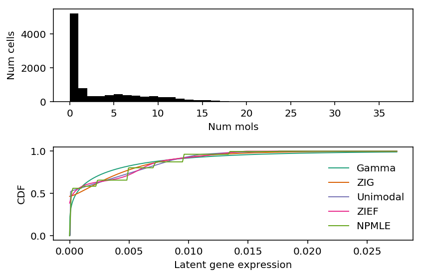
SLC25A5 (Solute carrier family 25 member 5) codes for a mitochrondrial membrane protein (Rocha et al. 2018), and is altered in Parkinson's disease
TXNDC17 (Thioredoxin domain-containing protein 17) appears to be involved in oxidative stress

Look at the fitted distributions for SLC25A5.

k = 'ENSG00000005022'
x = ipsc_counts.loc[:,k]
s = ipsc_counts.sum(axis=1)

plt.clf()
fig, ax = plt.subplots(2, 1)
fig.set_size_inches(6, 4)
ax[0].hist(x, bins=np.arange(x.max() + 1), color='k')
ax[0].set_xlabel('Num mols')
ax[0].set_ylabel('Num cells')

for c, k in zip(plt.get_cmap('Dark2').colors, ['Gamma', 'ZIG', 'Unimodal', 'ZIEF', 'NPMLE']):
  ax[1].plot(*getattr(scmodes.deconvolve, f'fit_{k.lower()}')(x, s), color=c, lw=1, label=k)
ax[1].set_xlabel('Latent gene expression')
ax[1].set_ylabel('CDF')
ax[1].legend(frameon=False)
fig.tight_layout()

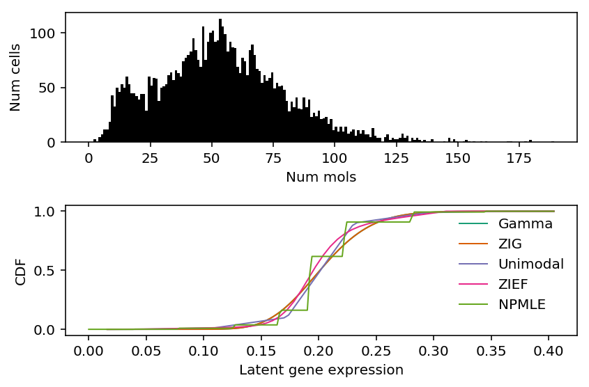
Conclusions:

When NPMLE does better than Gamma, unimodal does comparably well. The genes where this happens quite clearly exhibit unimodal gene expression.

Investigate Gamma vs. Point-Gamma in high-depth data

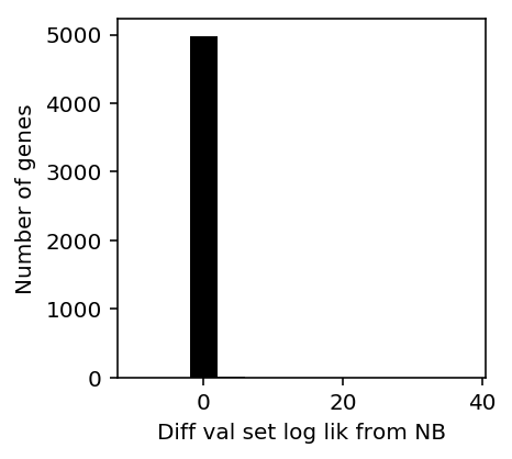
Look at the full benchmark results for NB vs. ZINB (only the GPU implementation is suitable for this).

ipsc_res = pd.read_csv('/project2/mstephens/aksarkar/projects/singlecell-modes/data/deconv-generalization/ipsc-gpu.txt.gz', index_col=0, sep='\t')

plt.clf()
plt.gcf().set_size_inches(3, 3)
h = plt.hist(ipsc_res['zinb'] - ipsc_res['nb'], color='k', bins=np.arange(-10, 40, 2))
plt.xlabel('Diff val set log lik from NB')
_ = plt.ylabel('Number of genes')

Print the histogram for inspection.

np.vstack((h[1][:-1], h[0])).T.astype(int)

array([[ -10,    0],
[  -8,    0],
[  -6,    0],
[  -4,    0],
[  -2, 4977],
[   0, 4973],
[   2,    2],
[   4,    3],
[   6,    0],
[   8,    0],
[  10,    0],
[  12,    0],
[  14,    1],
[  16,    0],
[  18,    0],
[  20,    0],
[  22,    0],
[  24,    0],
[  26,    0],
[  28,    1],
[  30,    0],
[  32,    0],
[  34,    0],
[  36,    0]])

Try to find a case in the full iPSC data where point-Gamma (ZINB) is required, by performing likelihood ratio tests against Gamma (NB). Use Bonferroni correction to control FWER.

lrt = st.chi2(1).sf(-2 * (ipsc_res['gamma'] - ipsc_res['point_gamma']))
ipsc_res[lrt < .05 / lrt.shape[0]]

gamma  point_gamma
gene
ENSG00000112530 -2017.717750 -1987.894352
ENSG00000129824 -1803.651932 -1789.106410

The two genes are PACRG and RPS4Y1. Look at the fitted distributions for these genes.

ipsc_counts = scmodes.dataset.ipsc(prefix='/project2/mstephens/aksarkar/projects/singlecell-qtl/data/',
                                   query=list(ipsc_res[lrt < .05 / lrt.shape[0]].index), return_df=True)

annotation = pd.read_csv('/project2/mstephens/aksarkar/projects/singlecell-qtl/data/scqtl-annotation.txt', sep='\t')
keep_samples = pd.read_csv('/project2/mstephens/aksarkar/projects/singlecell-qtl/data/quality-single-cells.txt', index_col=0, header=None, sep='\t')
s = annotation.loc[keep_samples.values.ravel(), 'mol_hs']

k = 'ENSG00000112530'
x = ipsc_counts.loc[:,k].values

plt.clf()
fig, ax = plt.subplots(2, 1)
fig.set_size_inches(6, 4)
ax[0].hist(x, bins=np.arange(x.max() + 1), color='k')
ax[0].set_title(gene_info.loc[k, 'name'])
ax[0].set_xlabel('Num mols')
ax[0].set_ylabel('Num cells')

for c, k in zip(plt.get_cmap('Dark2').colors, ['Gamma', 'ZIG', 'Unimodal', 'ZIEF', 'NPMLE']):
  ax[1].plot(*getattr(scmodes.deconvolve, f'fit_{k.lower()}')(x, s), color=c, lw=1, label=k)
ax[1].set_xlabel('Latent gene expression')
ax[1].set_ylabel('CDF')
ax[1].legend(frameon=False)
fig.tight_layout()

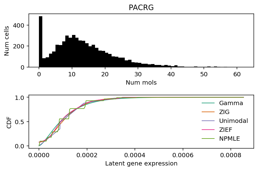
PACRG (Parkin coregulated gene) shares a promoter with PKRG (PARK2; Parkin). PARKIN is involved in a signaling pathway for mitochondria damage, and mitochrondrial damage appears to be relevant to neurodegenerative disease etiology (Alzheimer's disease and Parkinson's disease). Mitochrondrial damage could explain the bimodal distribution of PACRG in the iPSC data: the reprogramming protocol could induce oxidative stress on some of the cells, resulting in damage.

k = 'ENSG00000129824'
x = ipsc_counts.loc[:,k].values

plt.clf()
fig, ax = plt.subplots(2, 1)
fig.set_size_inches(6, 4)
ax[0].hist(x, bins=np.arange(x.max() + 1), color='k')
ax[0].set_title(gene_info.loc[k, 'name'])
ax[0].set_xlabel('Num mols')
ax[0].set_ylabel('Num cells')

for c, k in zip(plt.get_cmap('Dark2').colors, ['Gamma', 'ZIG', 'Unimodal', 'ZIEF', 'NPMLE']):
  ax[1].plot(*getattr(scmodes.deconvolve, f'fit_{k.lower()}')(x, s), color=c, lw=1, label=k)
ax[1].set_xlabel('Latent gene expression')
ax[1].set_ylabel('CDF')
ax[1].legend(frameon=False)
fig.tight_layout()

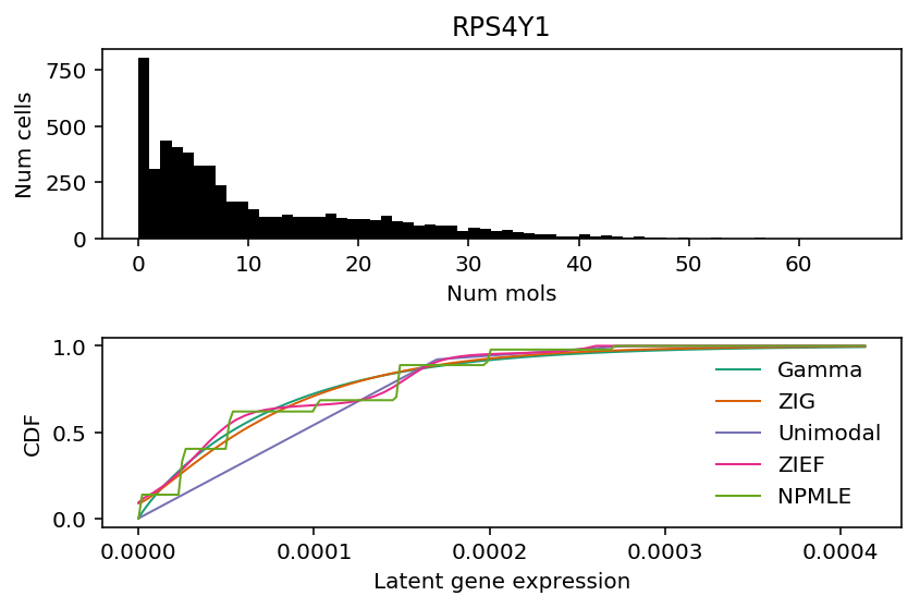
RPS4Y1 (Ribosomal protein S4, Y-linked) is on the Y chromosome, and therefore we should expect it to only be expressed in males. The homologous gene on the X chromosome (RPS4X) has a different coding sequence. Naively, sex-linkage should explain why this gene exhibits bimodal gene expression.

curl -OL 'http://ftp.1000genomes.ebi.ac.uk/vol1/ftp/technical/working/20130606_sample_info/20130606_sample_info.txt'

donor_info = pd.read_csv('/project2/mstephens/aksarkar/projects/singlecell-modes/data/20130606_sample_info.txt', sep='\t')

Count how many cells come from females.

prefix = '/project2/mstephens/aksarkar/projects/singlecell-qtl/data/'
annotations = pd.read_csv(f'{prefix}/scqtl-annotation.txt', sep='\t')
keep_samples = pd.read_csv(f'{prefix}/quality-single-cells.txt', sep='\t', index_col=0, header=None)
annotations = annotations.loc[keep_samples.values.ravel()]

annotations.merge(donor_info, left_on='chip_id', right_on='Sample')['Gender'].value_counts()

female    3109
male      2369
Name: Gender, dtype: int64

Look at the fitted ZINB distribution per-individual for this gene.

ipsc_log_mu = pd.read_csv('/project2/mstephens/aksarkar/projects/singlecell-qtl/data/density-estimation/design1/zi2-log-mu.txt.gz', sep=' ', index_col=0)
ipsc_log_phi = pd.read_csv('/project2/mstephens/aksarkar/projects/singlecell-qtl/data/density-estimation/design1/zi2-log-phi.txt.gz', sep=' ', index_col=0)
ipsc_logodds = pd.read_csv('/project2/mstephens/aksarkar/projects/singlecell-qtl/data/density-estimation/design1/zi2-logodds.txt.gz', sep=' ', index_col=0)

def point_gamma_cdf(grid, log_mu, log_phi, logodds):
  res = st.gamma(a=np.exp(-log_phi), scale=np.exp(log_mu + log_phi)).cdf(grid)
  res *= sp.expit(-logodds)
  res += sp.expit(logodds)
  return res

lam = ipsc_counts.values / annotations['mol_hs'].values.reshape(-1, 1)
grid = np.linspace(lam.min(), lam.max(), 1000)
cdfs = np.array([[point_gamma_cdf(grid,
                                  ipsc_log_mu.loc[j, k],
                                  ipsc_log_phi.loc[j, k],
                                  ipsc_logodds.loc[j, k])
                  for k in ipsc_log_mu]
                 for j in ipsc_counts.columns
                 if j != list(ipsc_log_mu.columns).index('NA18498')])

plt.clf()
fig, ax = plt.subplots(2, 1, sharex=True)
fig.set_size_inches(6, 4)
for a, F, k in zip(ax, cdfs, ipsc_counts.columns):
  for f in F:
    a.set_xlim(0, 2e-4)
    a.set_xticks(np.linspace(0, 2e-4, 3))
    a.plot(grid, f, c='k', lw=1, alpha=0.2)
  a.set_title(gene_info.loc[k, 'name'])
  a.set_ylabel('CDF')
ax[-1].set_xlabel('Latent gene expression')
fig.tight_layout()

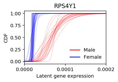
Plot the estimated RPS4Y1 latent gene expression, stratified by donor sex.

colors = {k: 'r' if v == 'male' else 'b' for k, v in
          donor_info.set_index('Sample')
          .filter(items=list(ipsc_log_mu.columns), axis=0)
          ['Gender']
          .iteritems()}
plt.clf()
plt.gcf().set_size_inches(3, 2)
for f, k in zip(cdfs[1], ipsc_log_mu.columns):
  plt.xlim(0, 2e-4)
  plt.xticks(np.linspace(0, 2e-4, 3))
  plt.plot(grid, f, lw=1, alpha=0.2, c=colors.get(k, 'k'))
  dummy = [plt.Line2D([0], [0], c='r'), plt.Line2D([0], [0], c='b')]
  plt.legend(dummy, ['Male', 'Female'], frameon=False)
  plt.title('RPS4Y1')
  plt.ylabel('CDF')
  plt.xlabel('Latent gene expression')

Synthetic mixtures

Read the results.

benchmark = {
  k: g.reset_index(level=0, drop=True) for k, g in
  (pd.read_csv('/project2/mstephens/aksarkar/projects/singlecell-modes/data/deconv-generalization/synthetic-mix-kl.txt.gz',
               sep='\t', index_col=[0, 1])
   .groupby(level=0))}

Read the data.

t_cells = scmodes.dataset.read_10x('/project2/mstephens/aksarkar/projects/singlecell-ideas/data/10xgenomics/cytotoxic_t/filtered_matrices_mex/hg19/', min_detect=0, return_df=True)
b_cells = scmodes.dataset.read_10x('/project2/mstephens/aksarkar/projects/singlecell-ideas/data/10xgenomics/b_cells/filtered_matrices_mex/hg19/', min_detect=0, return_df=True)
mix1, y1 = scmodes.dataset.synthetic_mix(t_cells, b_cells, min_detect=0.25)

cyto = scmodes.dataset.read_10x(prefix='/project2/mstephens/aksarkar/projects/singlecell-ideas/data/10xgenomics/cytotoxic_t/filtered_matrices_mex/hg19', return_df=True, min_detect=0)
naive = scmodes.dataset.read_10x(prefix='/project2/mstephens/aksarkar/projects/singlecell-ideas/data/10xgenomics/naive_cytotoxic/filtered_matrices_mex/hg19', return_df=True, min_detect=0)
mix2, y2 = scmodes.dataset.synthetic_mix(cyto, naive, min_detect=0.25)

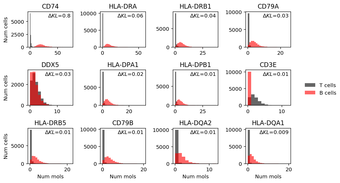
Look at T cell/B cell mix.

llik_diff = benchmark['cd8-cd19-mix']['npmle'] - benchmark['cd8-cd19-mix']['unimodal']
query = benchmark['cd8-cd19-mix'].loc[llik_diff[llik_diff > 0].sort_values(ascending=False).head(n=12).index].index.astype(int)
plt.clf()
fig, ax = plt.subplots(3, 4)
fig.set_size_inches(8, 5)
for a, k in zip(ax.ravel(), query):
  h = a.hist(mix1.loc[y1 == 1,mix1.columns[k]], bins=np.arange(mix1.iloc[:,k].max() + 1), color='k', alpha=0.6, label='T cells')
  a.hist(mix1.loc[y1 == 0,mix1.columns[k]], bins=np.arange(mix1.iloc[:,k].max() + 1), color='r', alpha=0.6, label='B cells')
  a.text(x=.95, y=.95,
         s=f"$\Delta KL$={llik_diff.iloc[k]:.1g}",
         horizontalalignment='right',
         verticalalignment='top',
         transform=a.transAxes)
  a.set_title(gene_info.loc[mix1.columns[k], 'name'] if mix1.columns[k] in gene_info.index else mix1.columns[k])
handles, labels = a.get_legend_handles_labels()
fig.legend(handles, labels, frameon=False, loc='center left', bbox_to_anchor=(1, 0.5))
for a in ax:
  a[0].set_ylabel('Num cells')
for a in ax.T:
  a[-1].set_xlabel('Num mols')
fig.tight_layout()

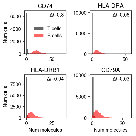
llik_diff = benchmark['cd8-cd19-mix']['npmle'] - benchmark['cd8-cd19-mix']['unimodal']
query = benchmark['cd8-cd19-mix'].loc[llik_diff[llik_diff > 0].sort_values(ascending=False).head(n=4).index].index.astype(int)
plt.clf()
fig, ax = plt.subplots(2, 2)
fig.set_size_inches(4, 4)
for a, k in zip(ax.ravel(), query):
  h = a.hist(mix1.loc[y1 == 1,mix1.columns[k]], bins=np.arange(mix1.iloc[:,k].max() + 1), color='k', alpha=0.6, label='T cells')
  a.hist(mix1.loc[y1 == 0,mix1.columns[k]], bins=np.arange(mix1.iloc[:,k].max() + 1), color='r', alpha=0.6, label='B cells')
  a.text(x=.95, y=.95,
         s=f"$\Delta l$={llik_diff.iloc[k]:.1g}",
         horizontalalignment='right',
         verticalalignment='top',
         transform=a.transAxes)
  a.set_title(gene_info.loc[mix1.columns[k], 'name'] if mix1.columns[k] in gene_info.index else mix1.columns[k])
ax[0, 0].legend(frameon=False, loc='center right')
for a in ax:
  a[0].set_ylabel('Num cells')
for a in ax.T:
  a[-1].set_xlabel('Num molecules')
fig.tight_layout()

Look cytotoxic/naive T cell mix.

llik_diff = benchmark['cyto-naive-t-mix']['npmle'] - benchmark['cyto-naive-t-mix']['unimodal']
query = benchmark['cyto-naive-t-mix'].loc[llik_diff[llik_diff > 0].sort_values(ascending=False).head(n=12).index].index
plt.clf()
fig, ax = plt.subplots(3, 4)
fig.set_size_inches(8, 5)
for a, k in zip(ax.ravel(), query):
  a.hist(mix2.loc[y1 == 1,k], bins=np.arange(mix2.loc[:,k].max() + 1), alpha=0.6, color='k', label='Cytotoxic T')
  a.hist(mix2.loc[y1 == 0,k], bins=np.arange(mix2.loc[:,k].max() + 1), alpha=0.6, color='r', label='Naive T')
  a.text(x=.95, y=.95,
         s=f"$\Delta KL$={llik_diff.loc[k]:.1g}",
         horizontalalignment='right',
         verticalalignment='top',
         transform=a.transAxes)
  a.set_title(gene_info.loc[k, 'name'] if k in gene_info.index else k)
handles, labels = a.get_legend_handles_labels()
fig.legend(handles, labels, frameon=False, loc='center left', bbox_to_anchor=(1, 0.5))
for a in ax:
  a[0].set_ylabel('Num cells')
for a in ax.T:
  a[-1].set_xlabel('Num mols')
fig.tight_layout()

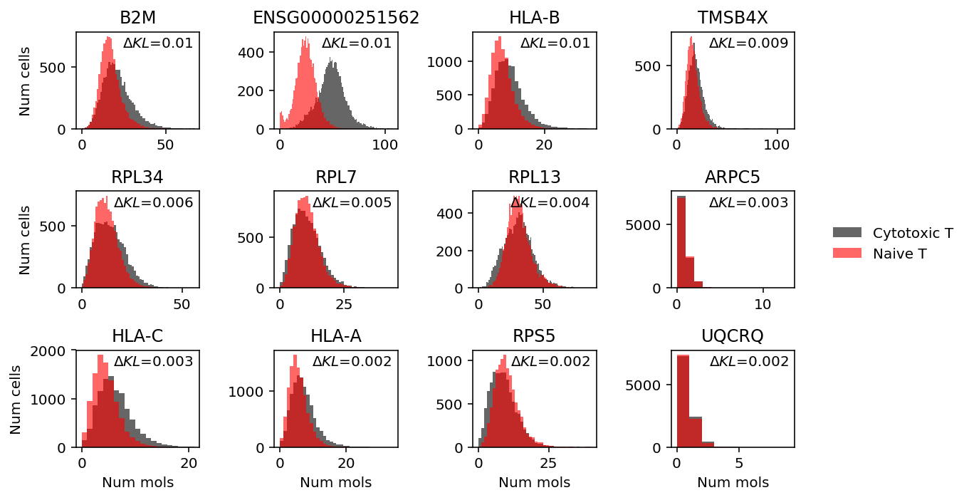
MALAT1 (Metastasis-associated lung adenocarcinoma transcript 1) is a lincRNA which appears to show tri-modal gene expression in this mixture. It is involved in T cell activation, through interaction with NF-κB (Zhao et al. 2016).

Heterogeneous populations

Read the results.

benchmark = {
  k: g.reset_index(level=0, drop=True) for k, g in
  (pd.read_csv('/project2/mstephens/aksarkar/projects/singlecell-modes/data/deconv-generalization/heterogeneous-kl.txt.gz',
               sep='\t', index_col=[0, 1])
   .groupby(level=0))}

Cortex

Fix the cortex count matrix (seems to break the parser in pandas).

import scmodes
work = scmodes.dataset.cortex('/project2/mstephens/aksarkar/projects/singlecell-ideas/data/zeisel-2015/GSE60361_C1-3005-Expression.txt.gz', return_df=True)
work.to_csv('/project2/mstephens/aksarkar/projects/singlecell-ideas/data/zeisel-2015/zeisel-2015.txt.gz', compression='gzip', sep='\t')

sbatch --partition=broadwl --mem=16G
#!/bin/bash
source activate scmodes
python <<EOF
<<fix-cortex>>
EOF

cortex_counts = pd.read_csv('/project2/mstephens/aksarkar/projects/singlecell-ideas/data/zeisel-2015/zeisel-2015.txt.gz', sep='\t', index_col=0)

Look at the fitted distribution for the genes where NPMLE does worst.

llik_diff = benchmark['cortex']['npmle'] - benchmark['cortex']['gamma']
llik_diff.sort_values().head(n=12)

Ttr           -3.136362
Hbb-bs        -3.032071
Hba-a2_loc1   -2.053220
Hba-a2_loc2   -1.985382
Sst           -1.842792
Apoe          -1.414460
Npy           -1.403264
Hbb-b2        -1.365434
Ccl3          -1.226098
Mgp           -1.198429
Acta2         -1.139285
Ptgds         -1.132885
dtype: float64

k = 'Ttr'
x = cortex_counts.loc[:,k].values
s = cortex_counts.sum(axis=1).values

plt.clf()
fig, ax = plt.subplots(2, 1)
fig.set_size_inches(6, 4)
ax[0].hist(x, bins=np.arange(0, x.max() + 1, 100), color='k')
ax[0].set_title(k.upper())
ax[0].set_xlabel('Num mols')
ax[0].set_ylabel('Num cells')

for c, k in zip(plt.get_cmap('Dark2').colors, ['Gamma', 'ZIG', 'Unimodal', 'ZIEF', 'NPMLE']):
  ax[1].plot(*getattr(scmodes.deconvolve, f'fit_{k.lower()}')(x, s), color=c, lw=1, label=k)
ax[1].set_xlabel('Latent gene expression')
ax[1].set_ylabel('CDF')
ax[1].legend(frameon=False)
fig.tight_layout()

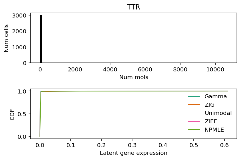
Look at the distribution of latent gene expression values (naively estimated) for TTR.

pd.Series((x / s)[x > 0]).describe()

count    90.000000
mean      0.059269
std       0.152847
min       0.000055
25%       0.000368
50%       0.003031
75%       0.008099
max       0.610003
dtype: float64

For these genes, more than 90% of the samples have observed count 0, so the optimal model appears to predict 0 for all samples.

Look at genes where ZIG does better than Gamma.

llik_diff = benchmark['cortex']['point_gamma'] - benchmark['cortex']['gamma']
query = benchmark['cortex'].loc[llik_diff[llik_diff > 0].sort_values(ascending=False).head(n=12).index].index
plt.clf()
fig, ax = plt.subplots(4, 3)
fig.set_size_inches(7, 5)
for a, k in zip(ax.ravel(), query):
  a.hist(cortex_counts.loc[:,k], bins=np.arange(cortex_counts.loc[:,k].max() + 1), color='k')
  a.text(x=.95, y=.95,
         s=f"$\Delta KL$={llik_diff.loc[k]:.1f}",
         horizontalalignment='right',
         verticalalignment='top',
         transform=a.transAxes)
  a.set_title(k.upper())
for y in range(ax.shape[0]):
  ax[y][0].set_ylabel('Num cells')
for x in range(ax.shape[1]):
  ax[-1][x].set_xlabel('Num mols')
fig.tight_layout()

Look at genes where unimodal shows greatest performance gain.

llik_diff = benchmark['cortex']['unimodal'] - benchmark['cortex']['gamma']
query = benchmark['cortex'].loc[llik_diff[llik_diff > 0].sort_values(ascending=False).head(n=12).index].index
plt.clf()
fig, ax = plt.subplots(4, 3)
fig.set_size_inches(7, 5)
for a, k in zip(ax.ravel(), query):
  a.hist(cortex_counts.loc[:,k], bins=np.arange(cortex_counts.loc[:,k].max() + 1), color='k')
  a.text(x=.95, y=.95,
         s=f"$\Delta KL$={llik_diff.loc[k]:.1f}",
         horizontalalignment='right',
         verticalalignment='top',
         transform=a.transAxes)
  a.set_title(k.upper())
for y in range(ax.shape[0]):
  ax[y][0].set_ylabel('Num cells')
for x in range(ax.shape[1]):
  ax[-1][x].set_xlabel('Num mols')
fig.tight_layout()

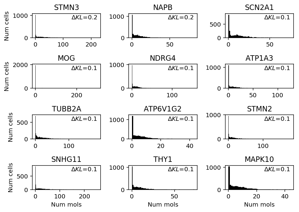
Show genes where NPMLE shows greatest performance gain.

llik_diff = benchmark['cortex']['npmle'] - benchmark['cortex']['gamma']
query = benchmark['cortex'].loc[llik_diff[llik_diff > 0].sort_values(ascending=False).head(n=12).index].index
plt.clf()
fig, ax = plt.subplots(4, 3)
fig.set_size_inches(7, 5)
for a, k in zip(ax.ravel(), query):
  a.hist(cortex_counts.loc[:,k], bins=np.arange(cortex_counts.loc[:,k].max() + 1), color='k')
  a.text(x=.95, y=.95,
         s=f"$\Delta KL$={llik_diff.loc[k]:.1f}",
         horizontalalignment='right',
         verticalalignment='top',
         transform=a.transAxes)
  a.set_title(k.upper())
for y in range(ax.shape[0]):
  ax[y][0].set_ylabel('Num cells')
for x in range(ax.shape[1]):
  ax[-1][x].set_xlabel('Num mols')
fig.tight_layout()

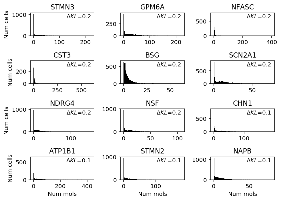
GPM6A (Glycoprotein m6a) appears to be required for mouse brain develoment, and is expressed in specific brain regions
SCN2A (Sodium channel, voltage-gated, type II, alpha) is needed for propagating actions potentials in neurons

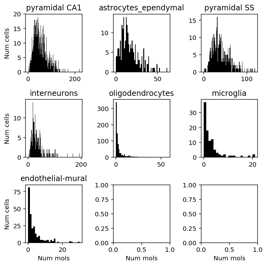
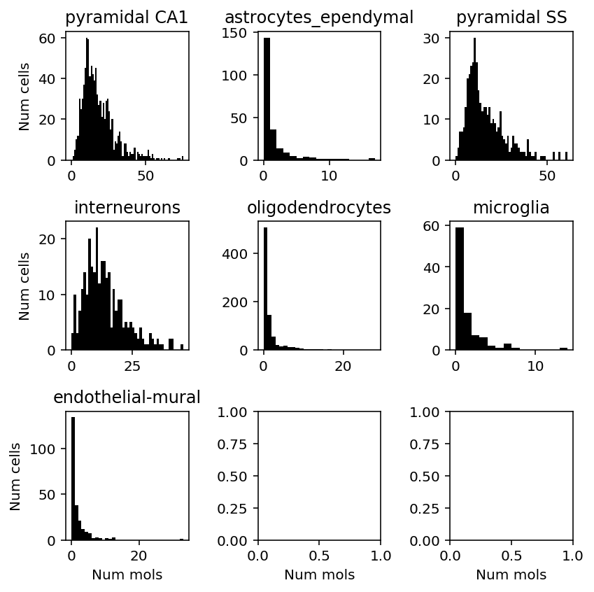
Stratify the gene expression of these genes by inferred cell type.

curl -sLO "https://storage.googleapis.com/linnarsson-lab-www-blobs/blobs/cortex/expression_mRNA_17-Aug-2014.txt"
gzip expression_mRNA_17-Aug-2014.txt

cortex_celltypes = (pd.read_csv('/project2/mstephens/aksarkar/projects/singlecell-ideas/data/zeisel-2015/expression_mRNA_17-Aug-2014.txt.gz', sep='\t', header=None, index_col=0, nrows=10)
                    .reset_index(drop=True)
                    .set_index(1))

plt.clf()
fig, ax = plt.subplots(3, 3)
fig.set_size_inches(6, 6)
for a, k in zip(ax.ravel(), set(cortex_celltypes.loc['level1class'])):
  x = cortex_counts.loc[(cortex_celltypes.loc['level1class'] == k).values, 'Gpm6a']
  a.hist(x, bins=np.arange(x.max() + 1), color='k')
  a.set_title(k)
for a in ax:
  a[0].set_ylabel('Num cells')
for a in ax.T:
  a[-1].set_xlabel('Num mols')
fig.tight_layout()

plt.clf()
fig, ax = plt.subplots(3, 3)
fig.set_size_inches(6, 6)
for a, k in zip(ax.ravel(), set(cortex_celltypes.loc['level1class'])):
  x = cortex_counts.loc[(cortex_celltypes.loc['level1class'] == k).values, 'Scn2a1']
  a.hist(x, bins=np.arange(x.max() + 1), color='k')
  a.set_title(k)
for a in ax:
  a[0].set_ylabel('Num cells')
for a in ax.T:
  a[-1].set_xlabel('Num mols')
fig.tight_layout()

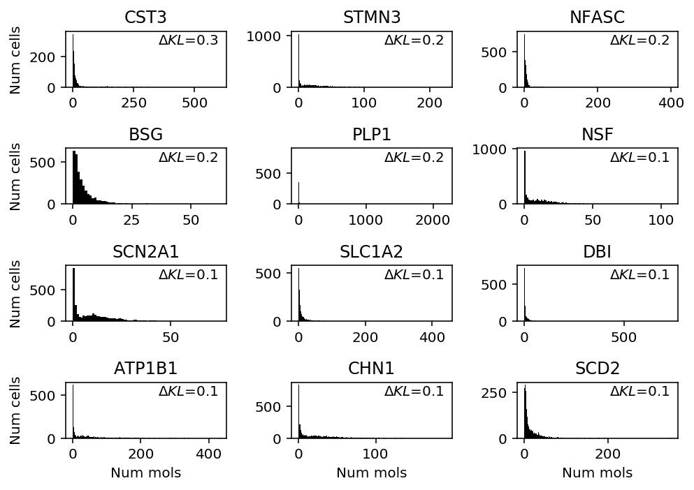
PBMCs

Read the PBMC data.

pbmcs_68k_counts = scmodes.dataset.read_10x('/project2/mstephens/aksarkar/projects/singlecell-ideas/data/10xgenomics/fresh_68k_pbmc_donor_a/filtered_matrices_mex/hg19/', return_df=True)

llik_diff = benchmark['pbmcs_68k']['npmle'] - benchmark['pbmcs_68k']['unimodal']
query = benchmark['pbmcs_68k'].loc[llik_diff[llik_diff > 0].sort_values(ascending=False).head(n=12).index].index
plt.clf()
fig, ax = plt.subplots(4, 3)
fig.set_size_inches(7, 5)
for a, k in zip(ax.ravel(), query):
  a.hist(pbmcs_68k_counts.loc[:,k], bins=np.arange(pbmcs_68k_counts.loc[:,k].max() + 1), color='k')
  a.text(x=.95, y=.95,
         s=f"$\Delta KL$={llik_diff.loc[k]:.2f}",
         horizontalalignment='right',
         verticalalignment='top',
         transform=a.transAxes)
  a.set_title(gene_info.loc[k, 'name'].upper())
for y in range(ax.shape[0]):
  ax[y][0].set_ylabel('Num cells')
for x in range(ax.shape[1]):
  ax[-1][x].set_xlabel('Num mols')
fig.tight_layout()

Distribution deconvolution examples

Table of Contents

Introduction

Setup

Results

Test

Metadata

Spike-in data

Homogeneous populations

Investigate Gamma vs. Point-Gamma in high-depth data

Synthetic mixtures

Heterogeneous populations

Cortex

PBMCs