Differential expression based on distribution deconvolution
Table of Contents
Introduction
For gene \(j\), consider the generative model for counts \(x_i, i=1, \ldots, n\):
\[ x_i \mid s_i, \lambda_i \sim \mathrm{Pois}(s_i \lambda_i) \]
\[ \lambda_i \sim g_{z_i}(\cdot) \]
where \(z_i\) denotes group membership. How do we use this model to test for differential expression?
Joyce Hsiao reports that commonly used count-based methods (deSeq2, edgeR) do not successfully control Type 1 error. But our preliminary results show a relatively simple count-based approach adequately controls Type 1 error here. There are two possible reasons:
- We are comparing much larger groups
- We are not shrinking dispersion parameters across genes
Setup
import numpy as np
import pandas as pd
import rpy2.robjects.packages
import rpy2.robjects.pandas2ri
import scipy.optimize as so
import scipy.stats as st
import scmodes
import scqtl.simple

mass = rpy2.robjects.packages.importr('MASS')
rpy2.robjects.pandas2ri.activate()
%matplotlib inline
%config InlineBackend.figure_formats = set(['retina'])
import matplotlib.pyplot as plt
plt.rcParams['figure.facecolor'] = 'w'
Methods
Deconvolution-based test
In the simplest case, suppose \(g_k = \delta_{\mu_k}\). Then,
\[ \hat\mu_k = \frac{\sum_i [z_i = k] x_i}{\sum_i [z_i = k] s_i} \]
This suggests a simple likelihood ratio test, comparing the null model
\[ x_i \sim \mathrm{Pois}(s_i \mu_0) \]
against an alternative model:
\[ x_i \sim \mathrm{Pois}(s_i \mu_{z_i}) \]
More generally, we can compare the null model:
\[ x_i \sim \mathrm{Pois}(s_i \lambda_i) \]
\[ \lambda_i \sim g_0(\cdot) \]
against an alternative model:
\[ x_i \sim \mathrm{Pois}(s_i \lambda_i) \]
\[ \lambda_i \sim g_{z_i}(\cdot) \]
In the general case, it will not be true that \(-2 \ln(l_0 - l_1) \sim \chi^2_1\). However, for the case where \(g\) is assumed to be Gamma distributed, it will be \(\chi^2_1\) or \(\chi^2_2\), depending on whether we allow dispersions to vary across groups also.
Realistic null simulation
Take a real homogeneous data set (sorted cells from Zheng et al. 2017), and randomly partition samples into two groups.
cd8 = scmodes.dataset.read_10x('/project2/mstephens/aksarkar/projects/singlecell-ideas/data/10xgenomics/cytotoxic_t/filtered_matrices_mex/hg19/', return_df=True)
s = cd8.sum(axis=1)
np.random.seed(0)
z = np.random.uniform(size=cd8.shape[0]) < 0.5
z.mean()
0.5071015770398668
Results
Point-mass deconvolution
First look at an idealized case where log-transform fails.
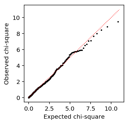
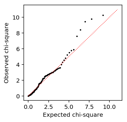
np.random.seed(0)
N = 100
onehot = np.zeros((2 * N, 2))
onehot[:N, 0] = 1
onehot[N:, 1] = 1
s = onehot.dot(np.array([1e5, 2e5]))
mu = 1e-5

llrs = []
pvals = []
for trial in range(1000):
  x = np.random.poisson(lam=s * mu)
  mu0 = x.sum() / s.sum()
  mu1 = x[:N].sum() / s[:N].sum()
  mu2 = x[N:].sum() / s[N:].sum()
  llr = st.poisson(mu=mu0).logpmf(x).sum() - st.poisson(mu=onehot.dot(np.array([mu1, mu2]))).logpmf(x).sum()
  llrs.append(llr)
llrs = np.array(llrs)
Look at the QQ plot.
plt.clf()
plt.gcf().set_size_inches(3, 3)
plt.scatter(st.chi2(1).ppf(np.linspace(0, 1, llrs.shape[0])), np.sort(-2 * llrs), c='k', s=2)
plt.plot([0, 11], [0, 11], c='r', lw=1, ls=':')
plt.xlabel('Expected chi-square')
plt.ylabel('Observed chi-square')
Text(0, 0.5, 'Observed chi-square')
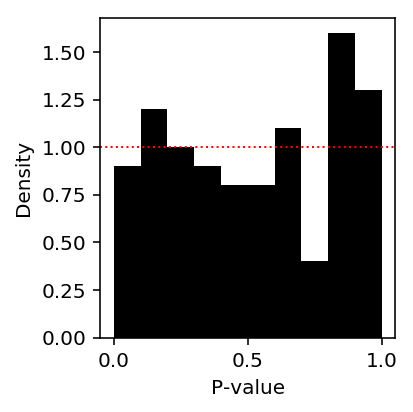
Look at the histogram of p-values.
plt.clf()
plt.gcf().set_size_inches(3, 3)
plt.hist(st.chi2(1).sf(-2 * llrs), np.linspace(0, 1, 11), density=True, color='black')
plt.axhline(y=1, lw=1, ls=':', c='r')
plt.xlabel('P-value')
plt.ylabel('Density')
plt.tight_layout()
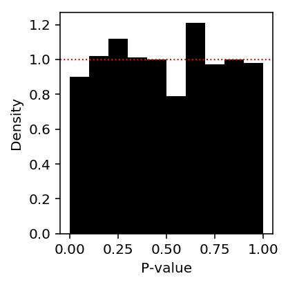
Deconvolve gene expression assuming \(g\) is a point mass (counts are marginally Poisson distributed). Naively, this should work because the data are informative about the mean.
def de(x, s, z):
  """Return LRT p-value

  x - counts (n,)
  s - size factors (n,)
  z - boolean group assignment (n,)

  """
  mu0 = x.sum() / s.sum()
  mu1 = x[z].sum() / s[z].sum()
  mu2 = x[~z].sum() / s[~z].sum()
  onehot = pd.get_dummies(z)
  llr = st.poisson(mu=mu0).logpmf(x).sum() - st.poisson(mu=onehot.dot(np.array([mu2, mu1]))).logpmf(x).sum()
  assert llr < 0
  return pd.Series({'mu0': mu0, 'mu1': mu1, 'mu2': mu2, 'llr': llr, 'p': st.chi2(1).sf(-2 * llr)})
de_res = cd8.apply(de, axis=0, args=(s, z)).T
plt.clf()
plt.gcf().set_size_inches(3, 3)
plt.hist(de_res.loc[:,'p'], np.linspace(0, 1, 11), density=True, color='black')
plt.axhline(y=1, lw=1, ls=':', c='r')
plt.xlabel('P-value')
plt.ylabel('Density')
plt.tight_layout()
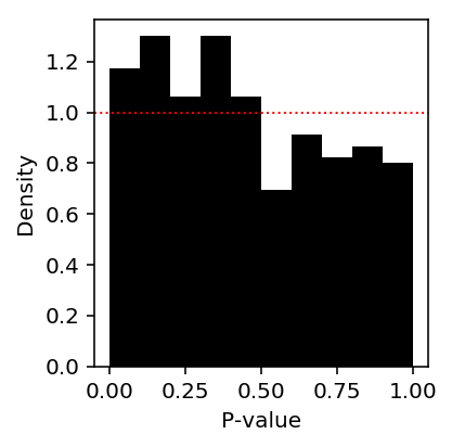
This result suggests that the sampling variance is not correctly estimated.
Gamma deconvolution
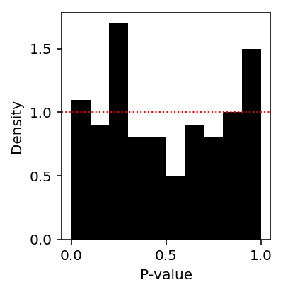
Deconvolve gene expression assuming group-specific Gammas under the alternative.
def fit_nb_collapse(x, s):
  """Return NB or Poisson solution, whichever is more sensible"""
  try:
    res = scqtl.simple.fit_nb(x, s)
  except:
    # Failure to converge
    res = scqtl.simple.fit_pois(x, s)
  # Converged to solution with large inverse overdispersion, so log likelihood
  # is nonsense
  if res[-1] > 0:
    res = scqtl.simple.fit_pois(x, s)
  return res

def de_nb(x, s, z):
  """Return LRT p-value

  x - counts (n,)
  s - size factors (n,)
  z - boolean group assignment (n,)

  """
  res0 = fit_nb_collapse(x, s)
  res1 = fit_nb_collapse(x[z], s[z])
  res2 = fit_nb_collapse(x[~z], s[~z])
  llr = res0[-1] - (res1[-1] + res2[-1])
  return pd.Series({'mu0': res0[0],
                    'mu1': res1[0],
                    'mu2': res2[0],
                    'llr': llr,
                    'p': st.chi2(2).sf(-2 * llr)})
de_nb_res = cd8.sample(n=100, axis=1, random_state=1).apply(de_nb, axis=0, args=(s, z)).T
Look at the histogram of p-values.
plt.clf()
plt.gcf().set_size_inches(3, 3)
plt.hist(de_nb_res['p'], np.linspace(0, 1, 11), density=True, color='black')
plt.axhline(y=1, lw=1, ls=':', c='r')
plt.xlabel('P-value')
plt.ylabel('Density')
plt.tight_layout()
Look at the QQ plot.
plt.clf()
plt.gcf().set_size_inches(3, 3)
plt.scatter(st.chi2(2).ppf(np.linspace(0, 1, de_nb_res.shape[0])), np.sort(-2 * de_nb_res['llr']), c='k', s=2)
plt.plot([0, 11], [0, 11], c='r', lw=1, ls=':')
plt.xlabel('Expected chi-square')
plt.ylabel('Observed chi-square')
Text(0, 0.5, 'Observed chi-square')
NB GLM
The Gamma deconvolution approach above corresponds to a generalized linear model:
\[ x_i \sim \mathrm{NB}(\mu_i, \phi_{z_i}) \]
\[ \ln(\mu_i) = \mathbf{z}_i + \ln s_i \]
where \(\mathrm{NB}(\mu, \phi)\) denotes the negative binomial distribution with mean \(\mu\) and variance \(\mu^2\phi\) and \(\mathbf{z}_i\) denotes a one-hot vector representing the group membership.
This level of flexibility in the dispersion parameters isn't readily available in existing GLM implementations. However, it is not obvious this level of flexibility is actually required.
If we consider the Gamma deconvolution approach essentially a \(t\)-test (mean and variance per group), we can compare the GLM approach with a single dispersion parameter \(\phi\) to a \(t\)-test with pooled variance.
def de_glm(x, s, z):
  f = rpy2.robjects.Formula('x ~ z + offset(log(s))')
  f.environment['x'] = x
  f.environment['z'] = pd.Series(z.astype(int))
  f.environment['s'] = s
  res = mass.glm_nb(f)
  pval = np.array(rpy2.robjects.r['coef'](rpy2.robjects.r['summary'](res)))[1,-1]
  return pval
de_glm_res = cd8.sample(n=100, axis=1, random_state=1).apply(de_glm, axis=0, args=(s, z)).T
Look at the histogram of p-values.
plt.clf()
plt.gcf().set_size_inches(3, 3)
plt.hist(de_glm_res, np.linspace(0, 1, 11), density=True, color='black')
plt.axhline(y=1, lw=1, ls=':', c='r')
plt.xlabel('P-value')
plt.ylabel('Density')
plt.tight_layout()
Debugging NB GLM
Figure out what happened in the DSC.
library(dplyr)
res = dscrutils::dscquery("/project2/mstephens/aksarkar/projects/dsc-log-fold-change/dsc/benchmark",
                          targets=c("data_poisthin.prop_null", "data_poisthin.nsamp", "type1error"), verbose=FALSE)
out = plyr::ddply(res, c("data_poisthin.prop_null", "data_poisthin.nsamp", "type1error.output.file"),
                  function (x) {readRDS(sprintf("/project2/mstephens/aksarkar/projects/dsc-log-fold-change/dsc/benchmark/%s.rds",
                                                x$type1error.output.file))$type_one_error})
out %>% group_by(data_poisthin.nsamp, data_poisthin.prop_null) %>% summarise(mean(V1), sd(V1))
| 100 | 0.9 | 0.0233333333333333 | 0.0114155814869796 |
| 100 | 1 | 0.0235 | 0.0104163333279998 |
| 500 | 0.9 | 0.0448888888888889 | 0.00838379781743461 |
| 500 | 1 | 0.0426 | 0.00783439709089205 |
head(out)
| 0.9 | 100 | type1error/datapoisthin1glmnb1type1error1 | 0.0133333333333333 |
| 0.9 | 100 | type1error/datapoisthin13glmnb2type1error2 | 0.0333333333333333 |
| 0.9 | 100 | type1error/datapoisthin17glmnb2type1error2 | 0.0244444444444444 |
| 0.9 | 100 | type1error/datapoisthin21glmnb2type1error2 | 0.0166666666666667 |
| 0.9 | 100 | type1error/datapoisthin25glmnb2type1error2 | 0.0244444444444444 |
| 0.9 | 100 | type1error/datapoisthin29glmnb2type1error2 | 0.05 |
Look at a false positive.
dat = readRDS("/project2/mstephens/aksarkar/projects/dsc-log-fold-change/dsc/benchmark/data_poisthin/data_poisthin_29.rds")
glm_res = readRDS("/project2/mstephens/aksarkar/projects/dsc-log-fold-change/dsc/benchmark/glm_nb/data_poisthin_29_glm_nb_2.rds")
parsed = data.frame(beta=dat$beta, betahat=glm_res$log_fold_change_est, shat=glm_res$s_hat, p=glm_res$pval)
y = dat$Y[10,]
s = colSums(dat$Y)
z = dat$X[,2]
fit = MASS::glm.nb(y ~ z + offset(log(s)))
summary(fit)
Call:
MASS::glm.nb(formula = y ~ z + offset(log(s)), init.theta = 0.3319585934,
    link = log)

Deviance Residuals:
    Min       1Q   Median       3Q      Max
-1.0912  -0.8465  -0.5935  -0.0329   3.6257

Coefficients:
            Estimate Std. Error z value Pr(>|z|)
(Intercept)  -7.6827     0.2914 -26.360  < 2e-16 ***
z            -1.2983     0.4794  -2.708  0.00676 **
---
Signif. codes:  0 ‘***’ 0.001 ‘**’ 0.01 ‘*’ 0.05 ‘.’ 0.1 ‘ ’ 1

(Dispersion parameter for Negative Binomial(0.332) family taken to be 1)

    Null deviance: 70.030  on 99  degrees of freedom
Residual deviance: 62.383  on 98  degrees of freedom
AIC: 184.42

Number of Fisher Scoring iterations: 1


              Theta:  0.332
          Std. Err.:  0.105

 2 x log-likelihood:  -178.425
Can we fix this by fitting group-specific dispersions?
dat = rpy2.robjects.r['readRDS']('/project2/mstephens/aksarkar/projects/dsc-log-fold-change/dsc/benchmark/data_poisthin/data_poisthin_29.rds')
X = np.array(dat.rx2('Y')).T
x = X[:,9]
s = X.sum(axis=1)
z = np.zeros(100).astype(bool)
z[:50] = 1
de_nb(x, s, z)
mu0    0.000292
mu1    0.000167
mu2    0.000404
llr   -4.349299
p      0.012916
dtype: float64
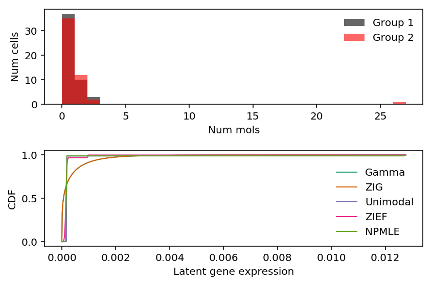
Look at this gene.
plt.clf()
fig, ax = plt.subplots(2, 1)
fig.set_size_inches(6, 4)
ax[0].hist(x[z], bins=np.arange(x.max() + 1), color='k', alpha=0.6, label='Group 1')
ax[0].hist(x[~z], bins=np.arange(x.max() + 1), color='r', alpha=0.6, label='Group 2')
ax[0].legend(frameon=False)
ax[0].set_xlabel('Num mols')
ax[0].set_ylabel('Num cells')

for c, k in zip(plt.get_cmap('Dark2').colors, ['Gamma', 'ZIG', 'Unimodal', 'ZIEF', 'NPMLE']):
  ax[1].plot(*getattr(scmodes.deconvolve, f'fit_{k.lower()}')(x, s), color=c, lw=1, label=k)
ax[1].set_xlabel('Latent gene expression')
ax[1].set_ylabel('CDF')
ax[1].legend(frameon=False)
fig.tight_layout()
Correct null model for Gamma deconvolution DE
Above we compared \(M_0\):
\[ x_i \mid s_i, \lambda_i \sim \mathrm{Poisson}(s_i \lambda_i) \]
\[ \lambda_i \mid \cdot \sim \mathrm{Gamma}(\mu_0, \phi_0) \]
to \(M_1\):
\[ x_i \mid s_i, \lambda_i \sim \mathrm{Poisson}(s_i \lambda_i) \]
\[ \lambda_i \mid \cdot \sim \mathrm{Gamma}(\mu_{z_i}, \phi_{z_i}) \]
However, this model comparison tests something more than just differential expression: \(M_1\) will fit the data better even if \(\mu_1 = \mu_2\), but \(\phi_1 \neq \phi_2\).
We really need to test \(\mu_1 \neq \mu_2\), allowing \(\phi_1 \neq \phi_2\). In principle, this could be achieved by computing a \(t\)-statistic; however, the necessary variance (standard error) is difficult to estimate.
Instead, we could test \(M_1\) against \(M'_0\):
\[ x_i \mid s_i, \lambda_i \sim \mathrm{Poisson}(s_i \lambda_i) \]
\[ \lambda_i \mid \cdot \sim \mathrm{Gamma}(\mu_0, \phi_{z_i}) \]
def nb_null_obj(theta, x, s, Z):
  mean = np.exp(theta[0])
  inv_disp = Z.dot(np.exp(theta[1:]))
  return -st.nbinom(n=inv_disp, p=1 / (1 + s * mean / inv_disp)).logpmf(x).sum()

def fit_nb_null(x, s, z):
  x, s = scqtl.simple.check_args(x, s)
  Z = pd.get_dummies(z).values
  opt = so.minimize(nb_null_obj, x0=[np.log(x.sum() / s.sum()), 10, 10], args=(x, s, Z), method='Nelder-Mead')
  if not opt.success:
    raise RuntimeError(opt.message)
  mean = np.exp(opt.x[0])
  inv_disp0 = np.exp(opt.x[1])
  inv_disp1 = np.exp(opt.x[2])
  nll = opt.fun
  return mean, inv_disp0, inv_disp1, -nll

def de_nb2(x, s, z):
  """Return LRT p-value

  x - counts (n,)
  s - size factors (n,)
  z - boolean group assignment (n,)

  """
  res0 = fit_nb_null(x, s, z)
  res1 = fit_nb_collapse(x[z], s[z])
  res2 = fit_nb_collapse(x[~z], s[~z])
  llr = res0[-1] - (res1[-1] + res2[-1])
  return pd.Series({'mu0': res0[0],
                    'inv_disp01': res0[1],
                    'inv_disp02': res0[2],
                    'mu1': res1[0],
                    'inv_disp1': res1[1],
                    'mu2': res2[0],
                    'inv_disp2': res2[1],
                    'llr': llr,
                    'p': st.chi2(2).sf(-2 * llr)})
Try on an example.
dat = rpy2.robjects.r['readRDS']('/project2/mstephens/aksarkar/projects/dsc-log-fold-change/dsc/benchmark/data_poisthin/data_poisthin_29.rds')
X = np.array(dat.rx2('Y')).T
x = X[:,9]
s = X.sum(axis=1)
z = np.zeros(100).astype(bool)
z[:50] = 1
res = fit_nb_null(x, s, z)
res
(0.0002303843030721306,
0.17676454746805434,
2.057596627861452,
-90.55969515068075)
de_nb2(x, s, z)
mu0           0.000230
inv_disp01    0.176765
inv_disp02    2.057597
mu1           0.000167
inv_disp1     4.781742
mu2           0.000404
inv_disp2     0.204504
llr          -2.118471
p             0.120215
dtype: float64