Single cell QTL mapping via sparse multiple regression
Table of Contents
Introduction
Sarkar et al. 2019 discovered mean and variance effect QTLs using a modular approach, first fitting the model \( \DeclareMathOperator\Gam{Gamma} \DeclareMathOperator\N{\mathcal{N}} \DeclareMathOperator\Poi{Poisson} \DeclareMathOperator\argmin{arg min} \newcommand\mf{\mathbf{F}} \newcommand\mg{\mathbf{G}} \newcommand\ml{\mathbf{L}} \newcommand\mx{\mathbf{X}} \newcommand\vb{\mathbf{b}} \newcommand\vl{\mathbf{l}} \newcommand\vx{\mathbf{x}} \)
\begin{align} x_{ij} \mid x_{i+}, \lambda_{ij} &\sim \Poi(x_{i+} \lambda_{ij})\\ \lambda_{ij} \mid \mu_{ij}, \phi_{ij}, \pi_{ij} &\sim \pi_{ij} \delta_0(\cdot) + (1 - \pi_{ij}) \Gam(\phi_{ij}^{-1}, \mu_{ij}^{-1} \phi_{ij}^{-1})\\ \ln \mu_{ij} &= (\ml \mf_\mu')_{ij}\\ \ln \phi_{ij} &= (\ml \mf_\phi')_{ij}\\ \operatorname{logit} \pi_{ij} &= (\ml \mf_\pi')_{ij}, \end{align}where
- \(x_{ij}\) is the number of molecules of gene \(j = 1, \ldots, p\) observed in cell \(i = 1, \ldots, n\)
- \(x_{i+} \triangleq \sum_j x_{ij}\) is the total number of molecules observed in sample \(i\)
- cells are taken from \(m\) donor individuals, \(\ml\) is \(n \times m\), and each \(\mf_{(\cdot)}\) is \(p \times m\)
- assignments of cells to donors (loadings) \(l_{ik} \in \{0, 1\}, k = 1, \ldots, m\) are known and fixed.
and then using a standard QTL mapping approach (e.g., Degner et al. 2012, McVicker et al. 2013) to discover genetic effects on gene expression mean \(E[\lambda_{ij}]\), dispersion \(\phi_{ij}\), and variance \(V[\lambda_{ij}]\). Critically, these quantities describe the distribution of latent gene expression, removing the effect of measurement noise (Sarkar and Stephens 2020).
This approach lost substantial power to detect effect on mean gene expression compared to bulk RNA-seq on the same (number of) samples (Banovich et al. 2018). One approach which might increase power would be to incorporate genotype into the expression model for gene \(j\)
\begin{align} \lambda_{i} &= \Gam(\phi_{i}^{-1}, \mu_{i}^{-1} \phi_{i}^{-1})\\ h^{-1}(\mu_{i}) &= (\ml\mg\vb_{\mu})_i + b_{\mu 0}\\ h^{-1}(\phi_{i}) &= (\ml\mg\vb_{\phi})_i + b_{\phi 0}, \end{align}where
- \(\mg\) denotes genotype (\(m \times s\))
- \(\vb_{\mu}\), \(\vb_{\phi}\) denote genetic effects (\(s \times 1)\)
- \(b_{\mu 0}\), \(b_{\phi 0}\) denote (scalar) intercepts
- \(h\) denotes a non-linearity mapping reals to positive reals (for practical purposes, we use the softplus function rather than the exponential function)
This approach would increase power by pooling samples across individuals with same (similar) genotypes, and is similar to previously proposed approaches (e.g., Rönnegård and Valdar 2011, Rönnegård and Valdar 2012). To fit this model for \(s > m\), we can further assume a sparsity-inducing prior
\begin{align} \vb_{\mu} &\sim \pi_{\mu} \delta_0(\cdot) + (1 - \pi_{\mu}) \N(0, \sigma_{\mu}^2)\\ \vb_{\phi} &\sim \pi_{\phi} \delta_0(\cdot) + (1 - \pi_{\phi}) \N(0, \sigma_{\phi}^2). \end{align}The prior is non-conjugate to the likelihood, so we perform variational inference (Blei et al. 2017), optimizing a stochastic objective (Kingma and Welling 2014, Rezende et al. 2014, Titsias and Lázaro-Gredilla 2014, Ranganath et al. 2014) via gradient descent. We use a local reparameterization (Kingma et al. 2015) to speed up convergence (Park et al. 2017).
Setup
Submitted batch job 1009091
import anndata
import gzip
import os
import numpy as np
import pandas as pd
import rpy2.robjects.pandas2ri
import rpy2.robjects.packages
import tabix
import time
import torch
import torch.utils.data as td
import txpred
import txpred.models.susie

rpy2.robjects.pandas2ri.activate()
susie = rpy2.robjects.packages.importr('susieR')
%matplotlib inline
%config InlineBackend.figure_formats = set(['retina'])
import colorcet
import matplotlib.pyplot as plt
plt.rcParams['figure.facecolor'] = 'w'
plt.rcParams['font.family'] = 'Nimbus Sans'
Results
Two stage approach
The motivation for restricting QTL mapping to 100kb windows in Sarkar et al. 2019 was to reduce the number of single SNP tests, and therefore increase the power to detect associations at a fixed FDR (intuitively, the BH procedure penalizes each test based on the total number of tests). Using multiple regression methods with Bayesian variable selection guarantees, we can simply avoid this issue. Read the estimated parameters.
log_mu1 = np.load('/scratch/midway2/aksarkar/ideas/mpebpm-ipsc-design-log-mu.npy')
neg_log_phi1 = np.load('/scratch/midway2/aksarkar/ideas/mpebpm-ipsc-design-neg-log-phi.npy')
logodds1 = np.load('/scratch/midway2/aksarkar/ideas/mpebpm-ipsc-design-logodds.npy')
(54, 9957)
Read the data/metadata.
y = anndata.read_h5ad('/project2/mstephens/aksarkar/projects/singlecell-ideas/data/ipsc/ipsc.h5ad')
Normalize the phenotype.
def qqnorm(x):
  return np.array(rpy2.robjects.r['qqnorm'](x)[0])

mean = (pd.DataFrame(np.exp(-np.log1p(np.exp(logodds1)) + log_mu1),
                     index=y.obs['chip_id'].unique(),
                     columns=y.var.index)
        .drop('NA18498', axis=0)
        .apply(qqnorm, axis=1))
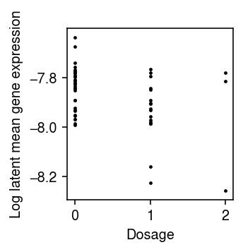
Fit a susie model (Wang et al. 2018) for each gene \(j\), regressing \(E[\lambda_{ij}]\) against cis-genotypes within the interval (TSS - 1MB, TES + 1MB).
window = 1e6
with gzip.open('/project2/mstephens/aksarkar/projects/singlecell-qtl/data/scqtl-mapping/yri-120-dosages.vcf.gz', 'rt') as f:
  for line in f:
    if line.startswith('#CHROM'):
      header = line.split()
      break
f = tabix.open('/project2/mstephens/aksarkar/projects/singlecell-qtl/data/scqtl-mapping/yri-120-dosages.vcf.gz')
for k, pheno in log_mean.iteritems():
  if y.var.loc[k, 'name'] != 'SKP1':
    continue
  try:
    info = y.var.loc[k]
    query = pd.DataFrame(list(f.query(f'chr{info["chr"][2:]}', info['start'] - int(window), info['start'] + int(window))))
    query.columns = header
    dose = query.filter(like='NA', axis=1).astype(float).T
    dose.columns = query['POS']
  except tabix.TabixError:
    continue
  dose, pheno = dose.align(pheno, axis=0, join='inner')
  fit = susie.susie(dose.values, pheno, L=1)
  break
plt.clf()
plt.gcf().set_size_inches(2.5, 2.5)
plt.scatter(dose["133515530"], pheno, c='k', s=2)
plt.xlabel('Dosage')
plt.ylabel('Log latent mean gene expression')
plt.tight_layout()
Single stage approach
Read the data.
y = anndata.read_h5ad('/project2/mstephens/aksarkar/projects/singlecell-ideas/data/ipsc/ipsc.h5ad')
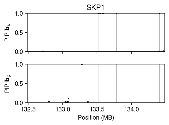
SKP1 was the top eQTL discovered in Sarkar et al. 2019. Extract the genotypes around the TSS.
y.var[y.var['name'] == 'SKP1']
chr      start        end  name strand      source
index
ENSG00000113558  hs5  133484633  133512729  SKP1      -  H. sapiens
tabix -h /project2/mstephens/aksarkar/projects/singlecell-qtl/data/scqtl-mapping/yri-120-dosages.vcf.gz chr5:$((133484633-1000000))-$((133484633+1000000)) | gzip >skp1.vcf.gz
Read the genotypes, and align it to the individuals with single cell measurements.
dat = pd.read_csv('/scratch/midway2/aksarkar/singlecell/skp1.vcf.gz', skiprows=2, sep='\t')
L = pd.get_dummies(y.obs['chip_id'])
x = dat.filter(like='NA', axis=1)
x.index = dat['POS']
x = x.sub(x.mean(axis=1), axis=0)
x = x.div(x.std(axis=1), axis=0)
L, x = L.align(x, axis=1, join='inner')
x.T.shape
(54, 5778)
Fit the sparse regression model.
torch.manual_seed(2)
# TODO: This doesn't get faster on the GPU. Utilization problem?
device = 'cpu:0'
data = td.DataLoader(
  td.TensorDataset(
    torch.tensor(L.values, dtype=torch.float, device=device),
    torch.tensor(y[:,y.var['name'] == 'SKP1'].X.A, dtype=torch.float, device=device),
    torch.tensor(y.obs['mol_hs'].values, dtype=torch.float, device=device)),
  batch_size=256, shuffle=True)
fit = (txpred.models.susie.PoisGamRegression(m=L.shape[1], p=x.shape[0])
       .fit(torch.tensor(x.values.T, dtype=torch.float, device=device), data, n_epochs=480, trace=True))
plt.clf()
fig, ax = plt.subplots(2, 1, sharex=True, sharey=True)
fig.set_size_inches(4, 3)
grid = np.array(x.index) / 1e6
pip = torch.sigmoid(fit.mean_prior.logits.detach()).numpy().ravel()
ax[0].scatter(grid[pip > 1e-2], pip[pip > 1e-2], s=2, c='k')
for t in grid[pip > .5]:
  for a in ax:
    a.axvline(x=t, lw=.5, c='0.7', zorder=-1)
ax[0].set_ylabel(r'PIP $\mathbf{b}_{\mu}$')
ax[0].set_xlim(grid.min(), grid.max())
ax[0].set_ylim(0, 1)
pip = torch.sigmoid(fit.inv_disp_prior.logits.detach()).numpy().ravel()
ax[1].scatter(grid[pip > 1e-2], pip[pip > 1e-2], s=2, c='k')
for t in grid[pip > .5]:
  for a in ax:
    a.axvline(x=t, lw=.5, c='0.7', zorder=-1)
ax[1].set_xlabel('Position (MB)')
ax[1].set_ylabel(r'PIP $\mathbf{b}_{\phi}$')
t = y.var.loc[y.var['name'] == 'SKP1', 'start'][0] / 1e6
for a in ax:
  a.axvline(x=t + .1, c='b', lw=.5, zorder=3)
  a.axvline(x=t - .1, c='b', lw=.5, zorder=3)
ax[0].set_title('SKP1')
fig.tight_layout()
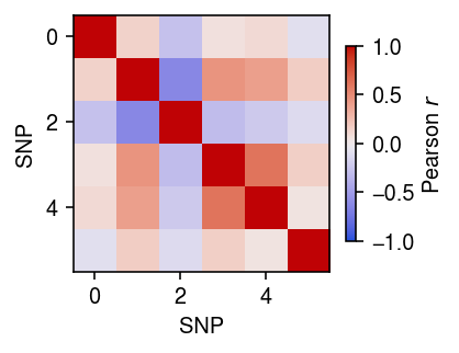
Look at the Pearson correlation between the SNPs with \(\mathrm{PIP}_{\mu} \triangleq p(b_{\mu j} \neq 0 \mid \cdot) > 0.5\) and those with \(\mathrm{PIP}_{\phi} > 0.5\).
plt.clf()
plt.gcf().set_size_inches(3, 3)
r = np.corrcoef(x[torch.sigmoid(fit.inv_disp_prior.logits.detach()).numpy().ravel() > 0.5],
            x[torch.sigmoid(fit.mean_prior.logits.detach()).numpy().ravel() > 0.5])
plt.imshow(r, cmap=colorcet.cm['coolwarm'], vmin=-1, vmax=1)
cb = plt.colorbar(shrink=0.5)
cb.set_label('Pearson $r$')
plt.xlabel('SNP')
plt.ylabel('SNP')
plt.tight_layout()
Fit a model for each gene, and output genes for which some mean effect or dispersion effect has PIP > 0.5.
<<imports>>
n_epochs = 80
window = 1e6
pip_thresh = 0.5
mean_effects = dict()
inv_disp_effects = dict()

y = anndata.read_h5ad('/project2/mstephens/aksarkar/projects/singlecell-ideas/data/ipsc/ipsc.h5ad')
L = pd.get_dummies(y.obs['chip_id'])

with gzip.open('/project2/mstephens/aksarkar/projects/singlecell-qtl/data/scqtl-mapping/yri-120-dosages.vcf.gz', 'rt') as f:
  for line in f:
    if line.startswith('#CHROM'):
      header = line.split()
      break

f = tabix.open('/project2/mstephens/aksarkar/projects/singlecell-qtl/data/scqtl-mapping/yri-120-dosages.vcf.gz')
for k, (chrom, start, end, name, _, _) in y.var.iterrows():
  try:
    query = pd.DataFrame(list(f.query(f'chr{chrom[2:]}', start - int(window), end + int(window))))
    if query.empty:
      print(f'skipping gene {k} (empty window)')
      continue
    query.columns = header
    x = query.filter(like='NA', axis=1).astype(float).align(L, axis=1, join='inner')[0]
  except tabix.TabixError:
    print(f'skipping gene {k} (TabixError)')
    continue
  print(f'fitting gene {k}')
  torch.manual_seed(1)
  data = td.DataLoader(
    td.TensorDataset(
      torch.tensor(L.values, dtype=torch.float),
      torch.tensor(y[:,k].X.A, dtype=torch.float),
      torch.tensor(y.obs['mol_hs'].values, dtype=torch.float)),
    batch_size=128, shuffle=True)
  fit = (txpred.models.susie.PoisGamRegression(m=L.shape[1], p=x.shape[0])
         .fit(torch.tensor(x.values.T, dtype=torch.float), data, n_epochs=n_epochs))

  alpha = torch.sigmoid(fit.mean_prior.logits.detach()).numpy()
  mu = fit.mean_prior.mean.detach().numpy()
  if (alpha > pip_thresh).any():
    mean_effects[(k, name, chrom)] = pd.DataFrame({
      'pos': query.loc[alpha > pip_thresh, 'POS'],
      'alpha': alpha[alpha > pip_thresh],
      'mu': mu[alpha > pip_thresh]})

  alpha = torch.sigmoid(fit.inv_disp_prior.logits.detach()).numpy()
  mu = fit.inv_disp_prior.mean.detach().numpy()
  if (alpha > pip_thresh).any():
    inv_disp_effects[(k, name, chrom)] = pd.DataFrame({
      'pos': query.loc[alpha > pip_thresh, 'POS'],
      'alpha': alpha[alpha > pip_thresh],
      'mu': mu[alpha > pip_thresh]})

if mean_effects:
  mean_df = (pd.concat(mean_effects)
             .reset_index(level=[0, 1, 2])
             .rename({f'level_{i}': k for i, k in enumerate(['gene', 'name', 'chr', 'pos'])}, axis=1))
  mean_df.to_csv('/scratch/midway2/aksarkar/singlecell/test/ipsc-mean-effects.txt.gz', sep='\t')
if inv_disp_effects:
  inv_disp_df = (pd.concat(inv_disp_effects)
                 .reset_index(level=[0, 1, 2])
                 .rename({f'level_{i}': k for i, k in enumerate(['gene', 'name', 'chr', 'pos'])}, axis=1))
  inv_disp_df.to_csv('/scratch/midway2/aksarkar/singlecell/test/ipsc-inv-disp-effects.txt.gz', sep='\t')
sbatch --partition=mstephens --mem=4G
#!/bin/bash
source activate singlecell
python /project2/mstephens/aksarkar/projects/singlecell-ideas/code/scqtl.py
Submitted batch job 1080540