Is eQTL analysis robust to removing some data points?
Table of Contents
Introduction
eQTL analysis is typically performed by fitting a series of simple linear regressions \( \DeclareMathOperator\N{\mathcal{N}} \DeclareMathOperator*\argmax{arg max} \newcommand\ones{\boldsymbol{1}} \newcommand\vx{\mathbf{x}} \newcommand\vw{\mathbf{w}} \newcommand\vy{\mathbf{y}} \)
\begin{equation} y_i \sim \N(x_i b, \sigma^2), \qquad i = 1, \ldots, n \end{equation}where \(y_i\) denotes the phenotype of individual \(i\), and \(x_i\) denotes the genotype at the SNP of interest (for simplicity, centered and scaled). Typically, one estimates \(\hat{b}\) and tests its statistical significance.
Broderick et al. 2020 demonstrate that such inferences can be not robust (e.g., changing statistical significance) to removing some of the data points, due to reasons other than heavy tailed errors, outliers, etc. The key ideas of their methodology are: (1) introduce a weight for each data point \(w_i\), so that dropping sample \(i\) corresponds to setting \(w_i = 0\); (2) write the inference problem (e.g., significance testing) as a functional \(\phi\) of the weighted data and an estimator \(\hat{b}(\cdot)\); and (3) write the question of robustness as an optimization problem
\begin{align} \vw^* &= \argmax_{\vw \in \mathcal{W}} \phi(\hat{b}(\vx, \vy, \vw), \vw) - \phi(\hat{b}(\vx, \vy, \ones), \ones)\\ &\approx \argmax_{\vw \in \mathcal{W}} \sum_i \left(\frac{\partial\phi}{\partial w_i} \Bigg\rvert_{\vw = \ones}\right) \end{align}where \(\mathcal{W}\) is some subset of all possible subsets of the data (e.g., all subsets of size \(m\)) and the last approximation is made via first-order Taylor expansion. Here, we play with this idea in the context of eQTL mapping, using simulations based on sample sizes used in real studies, and realistic effect sizes (Gusev et al. 2016, Wheeler et al. 2016). We also extend the methodology to the susie model (Wang et al. 2020).
Setup
import numpy as np
import pandas as pd
import scipy.stats as st
import sqlite3
import torch
%matplotlib inline
%config InlineBackend.figure_formats = set(['retina'])
import matplotlib.pyplot as plt
plt.rcParams['figure.facecolor'] = 'w'
plt.rcParams['font.family'] = 'Nimbus Sans'
Methods
Simple linear regression
def ols_bhat(x, y, w):
  assert x.shape == y.shape
  assert y.shape == w.shape
  xtx = x.T @ torch.diag(w.squeeze()) @ x
  bhat = torch.solve(x.T @ torch.diag(w.squeeze()) @ y, xtx)[0]
  s2 = torch.sum(w * (y - x @ bhat) ** 2) / (y.shape[0] - bhat.shape[0])
  se = torch.sqrt(s2 / xtx)
  return bhat, se

def ols_sign(bhat, se, w):
  # Important: we want to change sign from positive to negative
  return -bhat

def ols_fwer(bhat, se, w, alpha=.05 / 20000):
  """Indicator whether the test was significant at level 0.05 after Bonferroni
correction

  By default, assume p = 20,000 tests"""
  if bhat > 0:
    return -bhat / se + st.norm.ppf(alpha)
  else:
    return bhat / se - st.norm.ppf(alpha)

def ols_influence(x, y, phi, **kwargs):
  w = torch.ones_like(y, requires_grad=True)
  bhat, se = ols_bhat(x, y, w)
  assert torch.isfinite(bhat)
  phi = phi(bhat, se, w, **kwargs)
  phi.backward()
  with torch.no_grad():
    # Important: we need negative influence elsewhere
    return bhat.squeeze().numpy(), se.squeeze().numpy(), w.grad.squeeze().numpy()

def ols_prop_sign_change(x, y):
  bhat, se, influence = ols_influence(x, y, ols_sign)
  res = {'bhat': bhat, 'se': se}
  if bhat > 0:
    target = -bhat
    drop = np.where((np.cumsum(np.sort(influence)) < target))[0]
  else:
    target = bhat
    drop = np.where((np.cumsum(np.sort(-influence)) < target))[0]
  if drop.size > 0:
    n_drop = drop[0]
    res['n_drop'] = n_drop
    res['frac_drop'] = n_drop / y.shape[0]
    idx = np.argsort(influence)[:n_drop]
    res['drop'] = idx
    v = torch.ones_like(y)
    v[idx] = 0
    bhat1, se1 = ols_bhat(x, y, v)
    res['bhat1'] = bhat1
    res['se1'] = se1
  return res

def ols_prop_fwer_change(x, y, alpha=.05 / 20000):
  bhat, se, influence = ols_influence(x, y, ols_fwer, alpha=alpha)
  res = {'bhat': bhat, 'se': se, 'pval': min(st.norm.sf(bhat / se), st.norm.sf(-bhat / se))}
  if bhat > 0:
    target = -bhat / se + st.norm.sf(alpha / 2)
    drop = np.where((np.cumsum(np.sort(influence)) < target))[0]
  else:
    target = bhat / se - st.norm.sf(alpha / 2)
    drop = np.where((np.cumsum(np.sort(-influence)) < target))[0]
  if drop.size > 0:
    n_drop = drop[0]
    res['n_drop'] = n_drop
    res['frac_drop'] = n_drop / y.shape[0]
    idx = np.argsort(influence)[:n_drop]
    res['drop'] = idx
    v = torch.ones_like(y)
    v[idx] = 0
    bhat1, se1 = ols_bhat(x, y, v)
    res['bhat1'] = bhat1
    res['se1'] = se1
    res['pval1'] = st.norm.sf(bhat1 / se1)
  return res
eQTL simulation
Simulate genotypes at one SNP with allele frequency \(f\), and generate noise so that the PVE by the simulated genotype is as specified.
def simulate_easy(n, pve, seed=0):
  rng = np.random.default_rng(seed)
  x = rng.normal(size=n)
  # Important: fix b = 1
  e = rng.normal(scale=np.sqrt(((1 / pve) - 1)) * x.var(), size=n)
  y = x + e
  x -= x.mean()
  x /= x.std()
  y -= y.mean()
  return torch.tensor(x).unsqueeze(1), torch.tensor(y).unsqueeze(1)

def simulate(n, f, pve, seed=0):
  rng = np.random.default_rng(seed)
  x = rng.binomial(n=2, p=f, size=n).astype(float)
  # Important: fix b = 1
  e = rng.normal(scale=np.sqrt(((1 / pve) - 1)) * x.var(), size=n)
  y = x + e
  x -= x.mean()
  x /= x.std()
  y -= y.mean()
  return torch.tensor(x).unsqueeze(1), torch.tensor(y).unsqueeze(1)
Results
Sanity check
Check our implementation against the analytic expression (eq. 2.13).
x, y = simulate(n=100, f=0.25, pve=0.01, seed=0)
w = torch.ones_like(y, requires_grad=True)
bhat, se = ols_bhat(x, y, w)
bhat.backward()
torch.isclose(w.grad, x * (y - x @ bhat) / (x.T @ x)).all()
tensor(True)
Easy simulation
Simulate an example where the linear approximation is unlikely to be a problem.
x, y = simulate_easy(n=10000, pve=0.01)
bhat, se, influence = ols_influence(x, y, ols_sign)
n_drop = np.where(np.cumsum(np.sort(influence)) < -bhat)[0][0]
idx = np.argsort(influence)[:n_drop]
n_drop / x.shape[0]
0.0304
v = torch.ones_like(y, requires_grad=False)
v[idx] = 0
ols_bhat(x, y, v)
(tensor([[-0.0946]], dtype=torch.float64),
tensor([[0.0979]], dtype=torch.float64))
ols_prop_sign_change(x, y)
{'bhat': array(0.85542434),
'se': array(0.09851568),
'n_drop': 304,
'frac_drop': 0.0304,
'bhat1': tensor([[-0.0946]], dtype=torch.float64),
'se1': tensor([[0.0979]], dtype=torch.float64)}
Simulated eQTL
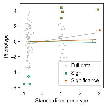
Simulate an eQTL with realistic allele frequency, sample size, and effect size. Report how many data points need to be removed to change the sign of \(\hat{b}\).
x, y = simulate(n=100, f=0.15, pve=0.02)
res = ols_prop_sign_change(x, y)
res
{'bhat': array(0.39178643),
'se': array(0.21633481),
'n_drop': 9,
'frac_drop': 0.09,
'drop': array([94, 97, 38, 89, 61, 40, 92, 37, 48]),
'bhat1': tensor([[-0.0382]], dtype=torch.float64),
'se1': tensor([[0.1885]], dtype=torch.float64)}
Report how many data points need to be removed to make the result not significant at level \(\alpha = 0.05\).
res1 = ols_prop_fwer_change(x, y, alpha=0.05)
res1
{'bhat': array(0.39178643),
'se': array(0.21633481),
'pval': 0.03506895996320592,
'n_drop': 6,
'frac_drop': 0.06,
'drop': array([94, 97, 38, 89, 37, 26]),
'bhat1': tensor([[0.0803]], dtype=torch.float64),
'se1': tensor([[0.2257]], dtype=torch.float64),
'pval1': array([[0.36104071]])}
cm = plt.get_cmap('Dark2')
plt.clf()
plt.gcf().set_size_inches(3, 3)

xx = x.squeeze().numpy() + np.random.normal(scale=0.1, size=x.shape[0])
plt.scatter(xx, y.squeeze().numpy(), c='0.7', s=2, label='Full data')
plt.plot([x.min(), x.max()], [x.min() * res['bhat'], x.max() * res['bhat']], c='0.7', lw=1)
for i, (r, l, m) in enumerate(zip([res, res1], ['Sign', 'Significance'], ['x', '+'])):
  plt.plot([x.min(), x.max()], [x.min() * r['bhat1'], x.max() * r['bhat1']], c=cm(i), lw=1)
  plt.scatter(xx[r['drop']], y[r['drop']], marker=m, s=16, c=cm(i), label=l)
plt.legend(handletextpad=0)
plt.xlabel('Standardized genotype')
plt.ylabel('Phenotype')
plt.tight_layout()
Simulate an eQTL with effect size equal to the median cis-heritability.
x, y = simulate(n=100, f=0.05, pve=0.16)
res = ols_prop_sign_change(x, y)
res
{'bhat': array(0.39748651), 'se': array(0.02987226)}
Real eQTLs
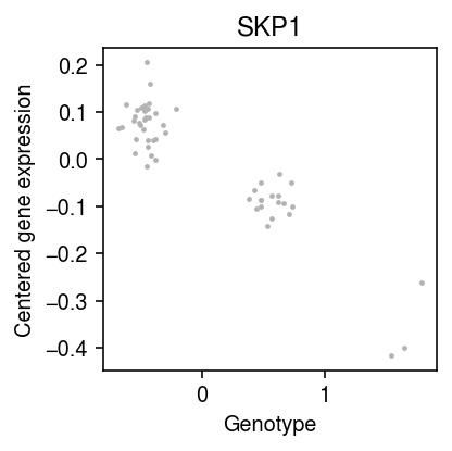
Look at the top eQTL in iPSC scRNA-seq (Sarkar et al. 2019).
log_mu = pd.read_csv('/project2/mstephens/aksarkar/projects/singlecell-qtl/data/density-estimation/design1/zi2-log-mu.txt.gz', sep=' ', index_col=0)
logodds = pd.read_csv('/project2/mstephens/aksarkar/projects/singlecell-qtl/data/density-estimation/design1/zi2-logodds.txt.gz', sep=' ', index_col=0)
genes = pd.read_csv('/project2/mstephens/aksarkar/projects/singlecell-qtl/data/scqtl-genes.txt.gz', sep='\t')

for x in (log_mu, logodds):
  del x['NA18498']

# Important: log(sigmoid(x)) = -softplus(-x)
log_mean = log_mu - np.log1p(np.exp(logodds))
with sqlite3.connect('/project2/mstephens/aksarkar/projects/singlecell-qtl/browser/browser.db') as conn:
  x = pd.read_sql('select * from mean_qtl_geno where gene = ?', con=conn, params=('ENSG00000113558',)).set_index('ind')['value']
y = log_mean.loc['ENSG00000113558']
y -= y.values.mean()
x -= x.values.mean()
x, y = x.align(y, join='inner')
res = ols_prop_fwer_change(torch.tensor(x.values.reshape(-1, 1)), torch.tensor(y.values.reshape(-1, 1)), alpha=0.005)
res
{'bhat': array(-0.19109817),
'se': array(0.01067698),
'pval': 6.096084570244492e-72}
plt.clf()
plt.gcf().set_size_inches(3, 3)
np.random.seed(2)
xx = x + np.random.normal(scale=0.1, size=x.shape[0])
plt.scatter(xx, y, color='0.7', s=2, label='Full data')
plt.xlabel('Genotype')
plt.ylabel('Centered gene expression')
plt.title('SKP1')
plt.tight_layout()
Look at a weaker eQTL.
mean_qtl_stats = pd.read_csv('/project2/mstephens/aksarkar/projects/singlecell-qtl/data/scqtl-mapping/zinb/mean.txt.gz', sep=' ', index_col=0)
mean_qtl_stats[mean_qtl_stats['p_beta'] < 2.5e-6].sort_values('p_beta', ascending=False).head()[['p_nominal', 'p_beta']]
p_nominal    p_beta
gene
ENSG00000134184  1.593470e-09  0.000002
ENSG00000105640  2.157150e-09  0.000002
ENSG00000182362  9.817790e-10  0.000002
ENSG00000145725  7.636840e-09  0.000002
ENSG00000142684  1.657690e-09  0.000002
k = 'ENSG00000134184'
with sqlite3.connect('/project2/mstephens/aksarkar/projects/singlecell-qtl/browser/browser.db') as conn:
  x = pd.read_sql('select * from mean_qtl_geno where gene = ?', con=conn, params=(k,)).set_index('ind')['value']
y = log_mean.loc[k]
x -= x.values.mean()
y -= y.values.mean()
x, y = x.align(y, join='inner')
res = ols_prop_fwer_change(torch.tensor(x.values.reshape(-1, 1)), torch.tensor(y.values.reshape(-1, 1)), alpha=0.005)
res
{'bhat': array(-0.51927837),
'se': array(0.07773376),
'pval': 1.1929436208959757e-11}