Hierarchical PMF
Table of Contents
Introduction
Consider the model \( \DeclareMathOperator\E{E} \DeclareMathOperator\Gam{Gamma} \DeclareMathOperator\KL{\mathcal{KL}} \DeclareMathOperator\Mult{Multinomial} \DeclareMathOperator\Pois{Poisson} \newcommand\mf{\mathbf{F}} \newcommand\ml{\mathbf{L}} \newcommand\mx{\mathbf{X}} \newcommand\va{\mathbf{a}} \newcommand\vb{\mathbf{b}} \newcommand\vs{\mathbf{s}} \newcommand\vl{\mathbf{l}} \newcommand\vf{\mathbf{f}} \)
\begin{align} x_{ij} \mid \lambda_{ij} &\sim \Pois(\lambda_{ij})\\ \lambda_{ij} &= (\ml\mf')_{ij}\\ l_{ik} &\sim \Gam(a_{lk}, b_{lk})\\ f_{jk} &\sim \Gam(a_{fk}, b_{fk}), \end{align}where the Gamma distributions are parameterized by shape and rate. Levitin et al. 2019 considered a variation of this model to model scRNA-seq data. One can use VBEM to estimate the posterior \(p(\ml, \mf \mid \mx, \va_l, \vb_l, \va_f, \vb_f)\) (Cemgil 2009). Here, we investigate alternative methods that do not rely on EM.
Setup
import numpy as np
import pandas as pd
import scipy.stats as st
import torch
import rpy2.robjects.packages
import rpy2.robjects.pandas2ri
rpy2.robjects.pandas2ri.activate()
%matplotlib inline
%config InlineBackend.figure_formats = set(['retina'])
import matplotlib.pyplot as plt
plt.rcParams['figure.facecolor'] = 'w'
plt.rcParams['font.family'] = 'Nimbus Sans'
Methods
VBEM
Consider the augmented model (Cemgil 2009)
\begin{align} x_{ij} &= \textstyle\sum_k z_{ijk}\\ z_{ijk} \mid l_{ik}, f_{jk} &\sim \Pois(l_{ik} f_{jk})\\ l_{ik} &\sim \Gam(a_{lk}, b_{lk})\\ f_{jk} &\sim \Gam(a_{fk}, b_{fk}). \end{align}VBEM updates for the variational parameters are analytic
\begin{align} q(z_{ij1}, \ldots, z_{ijK}) &= \Mult(x_{ij}, \pi_{ij1}, \ldots, \pi_{ijK})\\ \pi_{ijk} &\propto \exp(\E[\ln l_{ik}] + \E[\ln f_{jk}])\\ q(l_{ik}) &= \Gam(\textstyle \sum_j \E[z_{ijk}] + a_{lk}, \sum_j \E[f_{jk}] + b_{lk})\\ &\triangleq \Gam(\alpha_{lik}, \beta_{lk})\\ q(f_{jk}) &= \Gam(\textstyle \sum_i \E[z_{ijk}] + a_{fk}, \sum_i \E[l_{ik}] + b_{fk})\\ &\triangleq \Gam(\alpha_{fjk}, \beta_{fk}), \end{align}where the expectations
\begin{align} \E[z_{ijk}] &= x_{ij} \pi_{ijk}\\ \E[l_{ik}] &= \alpha_{lik} / \beta_{lk}\\ \E[\ln l_{ik}] &= \psi(\alpha_{lik}) - \ln \beta_{lk}\\ \E[f_{jk}] &= \alpha_{fjk} / \beta_{fk}\\ \E[\ln f_{jk}] &= \psi(\alpha_{fjk}) - \ln \beta_{fk}, \end{align}and \(\psi\) denotes the digamma function. The ELBO
\begin{multline} \ell = \sum_{i, j} \left[ \sum_k \Big[ \E[z_{ijk}] (\E[\ln l_{ik}] + \E[\ln f_{jk}] - \ln \pi_{ijk}) - \E[l_{ik}]\E[f_{jk}] \Big] - \ln\Gamma(x_{ij} + 1)\right]\\ + \sum_{i, k} \left[ (a_{lk} - \alpha_{lik}) \E[\ln l_{ik}] - (b_{lk} - \beta_{lk}) \E[l_{ik}] + a_{lk} \ln b_{lk} - \alpha_{lik} \ln \beta_{lk} - \ln\Gamma(a_{lk}) + \ln\Gamma(\alpha_{lik})\right]\\ + \sum_{j, k} \left[ (a_{fk} - \alpha_{fjk}) \E[\ln f_{jk}] - (b_{fk} - \beta_{fk}) \E[f_{jk}] + a_{fk} \ln b_{fk} - \alpha_{fjk} \ln \beta_{fk} - \ln\Gamma(a_{fk}) + \ln\Gamma(\alpha_{fjk})\right]. \end{multline}Letting \(t_{ij} \triangleq \sum_k \exp(\E[\ln l_{ik}] + \E[\ln f_{jk}])\), and plugging in \(\E[z_{ijk}], \pi_{ijk}\),
\begin{gather} \sum_{i, j, k} \E[z_{ijk}] (\E[\ln l_{ik}] + \E[\ln f_{jk}] - \ln \pi_{ijk}) = \sum_{i, j} x_{ij} \ln t_{ij}\\ \sum_i \E[z_{ijk}] = \exp(\E[\ln f_{jk}]) \sum_i \frac{x_{ij}}{t_{ij}} \exp(\E[\ln l_{ik}])\\ \sum_j \E[z_{ijk}] = \exp(\E[\ln l_{ik}]) \sum_j \frac{x_{ij}}{t_{ij}} \exp(\E[\ln f_{jk}]). \end{gather}Updates for \(b_{lk}, b_{fk}\) are analytic:
\begin{align} \frac{\partial \ell}{\partial b_{lk}} &= \sum_{i} \left[\frac{a_{lk}}{b_{lk}} - \E[l_{ik}]\right] = 0\\ b_{lk} &:= \frac{n a_{lk}}{\sum_{i} \E[l_{ik}]}\\ \frac{\partial \ell}{\partial b_{fk}} &= \sum_{j} \left[\frac{a_{fk}}{b_{fk}} - \E[f_{jk}]\right] = 0\\ b_{fk} &:= \frac{p a_{fk}}{\sum_{j} \E[f_{jk}]}, \end{align}as are gradients for \(a_{lk}, a_{fk}\):
\begin{align} \frac{\partial \ell}{\partial a_{lk}} &= \sum_{i} \Big[\E[\ln l_{ik}] + \ln b_{lk} - \psi(a_{lk})\Big]\\ \frac{\partial^2 \ell}{\partial a_{lk}^2} &= -\psi^{(1)}(a_{lk})\\ \frac{\partial \ell}{\partial a_{fk}} &= \sum_{j} \Big[\E[\ln f_{jk}] + \ln b_{fk} - \psi(a_{fk})\Big]\\ \frac{\partial^2 \ell}{\partial a_{fk}^2} &= -\psi^{(1)}(a_{fk}), \end{align}where \(\psi^{(1)}\) denotes the trigamma function.
class PMFVBEM(torch.nn.Module):
  def __init__(self, n, p, k):
    super().__init__()
    self.alpha_l = torch.nn.Parameter(torch.exp(torch.randn([n, k])))
    self.beta_l = torch.nn.Parameter(torch.exp(torch.randn([1, k])))
    self.alpha_f = torch.nn.Parameter(torch.exp(torch.randn([p, k])))
    self.beta_f = torch.nn.Parameter(torch.exp(torch.randn([1, k])))
    self.a_l = torch.nn.Parameter(torch.ones([1, k]))
    self.b_l = torch.nn.Parameter(torch.ones([1, k]))
    self.a_f = torch.nn.Parameter(torch.ones([1, k]))
    self.b_f = torch.nn.Parameter(torch.ones([1, k]))

  @torch.no_grad()
  def elbo(self, x):
    """ELBO wrt q(l_{ik}) q(f_{jk}), i.e. integrating out z_{ijk}"""
    q_l = torch.distributions.Gamma(self.alpha_l, self.beta_l)
    q_f = torch.distributions.Gamma(self.alpha_f, self.beta_f)
    kl_l = torch.distributions.kl.kl_divergence(q_l, torch.distributions.Gamma(self.a_l, self.b_l)).sum()
    kl_f = torch.distributions.kl.kl_divergence(q_f, torch.distributions.Gamma(self.a_f, self.b_f)).sum()
    # TODO: multiple samples?
    l = q_l.rsample()
    f = q_f.rsample()
    err = torch.distributions.Poisson(l @ f.T).log_prob(x).sum()
    elbo = err - kl_l - kl_f
    return elbo

  def _pm(self, x):
    pm_l = self.alpha_l / self.beta_l
    pm_ln_l = torch.digamma(self.alpha_l) - torch.log(self.beta_l)
    pm_f = self.alpha_f / self.beta_f
    pm_ln_f = torch.digamma(self.alpha_f) - torch.log(self.beta_f)
    t = x / (torch.exp(pm_ln_l) @ torch.exp(pm_ln_f).T)
    return pm_l, pm_ln_l, pm_f, pm_ln_f, t

  def elbo_z(self, x):
    """ELBO wrt q(l_{ik}) q(f_{jk}) q(z_{ijk})"""
    pm_l, pm_ln_l, pm_f, pm_ln_f, _ = self._pm(x)
    ret = (x * torch.log(torch.exp(pm_ln_l) @ torch.exp(pm_ln_f).T)
           - pm_l @ pm_f.T
           - torch.lgamma(x + 1)).sum()
    ret += ((self.a_l - self.alpha_l) * pm_ln_l
            - (self.b_l - self.beta_l) * pm_l
            + self.a_l * torch.log(self.b_l)
            - self.alpha_l * torch.log(self.beta_l)
            - torch.lgamma(self.a_l)
            + torch.lgamma(self.alpha_l)).sum()
    ret += ((self.a_f - self.alpha_f) * pm_ln_f
            - (self.b_f - self.beta_f) * pm_f
            + self.a_f * torch.log(self.b_f)
            - self.alpha_f * torch.log(self.beta_f)
            - torch.lgamma(self.a_f)
            + torch.lgamma(self.alpha_f)).sum()
    assert torch.isfinite(ret)
    assert ret <= 0
    return ret

  @torch.no_grad()
  def fit(self, x, num_epochs, eps=1e-15, step=1):
    self.trace = []
    self.trace2 = []
    for i in range(num_epochs):
      self.trace.append(-self.elbo(x).cpu().numpy())
      self.trace2.append(-self.elbo_z(x).cpu().numpy())
      obj = self.elbo_z(x).cpu().numpy()
      # Cemgil 2009, Alg. 1
      # Important: this optimizes elbo_z, not elbo
      pm_l, pm_ln_l, pm_f, pm_ln_f, t = self._pm(x)
      self.alpha_l.data = torch.exp(pm_ln_l) * (t @ torch.exp(pm_ln_f)) + self.a_l
      self.beta_l.data = pm_f.sum(dim=0) + self.b_l
      pm_l, pm_ln_l, pm_f, pm_ln_f, t = self._pm(x)
      self.alpha_f.data = torch.exp(pm_ln_f) * (torch.exp(pm_ln_l).T @ t).T + self.a_f
      self.beta_f.data = pm_l.sum(dim=0) + self.b_f
      pm_l, pm_ln_l, pm_f, pm_ln_f, _ = self._pm(x)
      self.a_l.data += step * (pm_ln_l + torch.log(self.b_l) - torch.digamma(self.a_l)).sum(dim=0) / torch.polygamma(1, self.a_l)
      torch.clamp(self.a_l, min=eps)
      self.b_l.data = pm_l.shape[0] * self.a_l / pm_l.sum(dim=0)
      self.a_f.data += step * (pm_ln_f + torch.log(self.b_f) - torch.digamma(self.a_f)).sum(dim=0) / torch.polygamma(1, self.a_f)
      torch.clamp(self.a_f, min=eps)
      self.b_f.data = pm_f.shape[0] * self.a_f / pm_f.sum(dim=0)
    return self
Newton-Raphson
Alternatively, one could plug in \(\E[z_{ijk}], \pi_{ijk}\) and then optimize the ELBO with respect to \(\alpha_{lik}, \beta_{lk}, \alpha_{fjk}, \beta_{fk}, a_{lk}, b_{lk}, a_{fk}, b_{fk}\) using one-dimensional Newton-Raphson updates. To prototype this approach, we use automatic differentiation to get the first and second derivatives.
class PMFN(torch.nn.Module):
  def __init__(self, n, p, k):
    super().__init__()
    self.alpha_l = torch.nn.Parameter(torch.exp(torch.randn([n, k])))
    self.beta_l = torch.nn.Parameter(torch.exp(torch.randn([1, k])))
    self.alpha_f = torch.nn.Parameter(torch.exp(torch.randn([p, k])))
    self.beta_f = torch.nn.Parameter(torch.exp(torch.randn([1, k])))
    self.a_l = torch.nn.Parameter(torch.ones([1, k]))
    self.b_l = torch.nn.Parameter(torch.ones([1, k]))
    self.a_f = torch.nn.Parameter(torch.ones([1, k]))
    self.b_f = torch.nn.Parameter(torch.ones([1, k]))

  @torch.no_grad()
  def elbo(self, x):
    q_l = torch.distributions.Gamma(self.alpha_l, self.beta_l)
    q_f = torch.distributions.Gamma(self.alpha_f, self.beta_f)
    kl_l = torch.distributions.kl.kl_divergence(q_l, torch.distributions.Gamma(self.a_l, self.b_l)).sum()
    kl_f = torch.distributions.kl.kl_divergence(q_f, torch.distributions.Gamma(self.a_f, self.b_f)).sum()
    # TODO: multiple samples?
    l = q_l.rsample()
    f = q_f.rsample()
    err = torch.distributions.Poisson(l @ f.T).log_prob(x).sum()
    elbo = err - kl_l - kl_f
    return elbo

  def elbo_z(self, x):
    pm_l = (self.alpha_l / self.beta_l)
    exp_pm_ln_l = torch.exp(torch.digamma(self.alpha_l) - torch.log(self.beta_l))
    pm_f = (self.alpha_f / self.beta_f)
    exp_pm_ln_f = torch.exp(torch.digamma(self.alpha_f) - torch.log(self.beta_f))
    temp = exp_pm_ln_l @ exp_pm_ln_f.T
    ret = (x * torch.log(temp) - pm_l @ pm_f.T - torch.lgamma(x + 1)).sum()
    ret += ((self.a_l - self.alpha_l) * torch.log(exp_pm_ln_l)
            - (self.b_l - self.beta_l) * pm_l
            + self.a_l * torch.log(self.b_l)
            - self.alpha_l * torch.log(self.beta_l)
            - torch.lgamma(self.a_l)
            + torch.lgamma(self.alpha_l)).sum()
    ret += ((self.a_f - self.alpha_f) * torch.log(exp_pm_ln_f)
            - (self.b_f - self.beta_f) * pm_f
            + self.a_f * torch.log(self.b_f)
            - self.alpha_f * torch.log(self.beta_f)
            - torch.lgamma(self.a_f)
            + torch.lgamma(self.alpha_f)).sum()
    assert not torch.isnan(ret)
    assert torch.isfinite(ret)
    assert ret <= 0
    return ret

  def _update(self, x, par, step=1, eps=1e-15):
    """Newton-Raphon update"""
    for i in range(par.shape[0]):
      for k in range(par.shape[1]):
        # Important: this optimizes elbo_z, not elbo
        d = torch.autograd.grad(self.elbo_z(x), par, create_graph=True)[0]
        d2 = torch.autograd.grad(d[i,k], par)[0]
        with torch.no_grad():
          par.data[i,k] -= step * d[i,k] / (d2[i,k] + eps)
          par.data[i,k] = torch.clamp(par.data[i,k], min=eps)

  def fit(self, x, num_epochs, step=1):
    self.trace = []
    self.trace2 = []
    for t in range(num_epochs):
      # TODO: update order probably matters
      for par in self.parameters():
        if par.requires_grad:
          self._update(x, par, step=step)
      self.trace.append(-self.elbo(x).cpu().numpy())
      with torch.no_grad():
        self.trace2.append(-self.elbo_z(x).cpu().numpy())
    return self
Pathwise gradient
In the original model, the ELBO
\begin{equation} \ell = \sum_{i,j} \E[\ln p(x_{ij} \mid \ml, \mf)] - \KL(q(\ml) \Vert p(\ml)) - \KL(q(\mf) \Vert p(\mf)). \end{equation}The KL terms are analytic; however, the first expectation is not (unlike for the approach described above, which made a variational approximation on \(z\)). In this case, one can still optimize the ELBO using the pathwise gradient (reviewed by Mohamed et al. 2020) and gradient descent. Briefly,
\begin{align} \nabla \textstyle \sum_{i,j} \E[\ln p(x_{ij} \mid \ml, \mf)] &\approx \frac{1}{S} \sum_{s=1}^S \sum_{i,j} \nabla \ln p(x_{ij} \mid \ml^{(s)}, \mf^{(s)}), \quad \ml^{(s)} \sim q(\ml), \mf^{(s)} \sim q(\mf)\\ &= \frac{1}{S} \sum_{s=1}^S \sum_{i,j} \nabla \ln p(x_{ij} \mid h_{\ml}(\epsilon_{\ml}^{(s)}), h_{\mf}(\epsilon_{\ml}^{(s)})), \quad \epsilon_{\ml}^{(s)} \sim \Gam(1, 1), \epsilon_{\mf}^{(s)} \sim \Gam(1, 1), \end{align}where \(\epsilon_{\ml}, \epsilon_{\mf}\) are matrices with elements following a standard Gamma distribution and \(h_{\ml}, h_{\mf}\) are differentiable, element-wise functions of the sampled elements and the variational parameters. The difference between the two lower bounds is
\begin{equation} \sum_{i, j} x_{ij} \Big[ \E[\ln(\textstyle \sum_k l_{ik} f_{jk})] - \ln (\sum_k \exp(\E[\ln l_{ik}] + \E[\ln f_{jk}])) \Big], \end{equation}which may always be non-negative (intuitively, it seems to follow from Jensen’s inequality). It is not clear that the local optima of the two lower bounds are the same.
class PMFGD(torch.nn.Module):
  def __init__(self, n, p, k):
    super().__init__()
    self.alpha_l = torch.nn.Parameter(torch.exp(torch.randn([n, k])))
    self.beta_l = torch.nn.Parameter(torch.exp(torch.randn([1, k])))
    self.alpha_f = torch.nn.Parameter(torch.exp(torch.randn([p, k])))
    self.beta_f = torch.nn.Parameter(torch.exp(torch.randn([1, k])))
    self.a_l = torch.nn.Parameter(torch.ones([1, k]))
    self.b_l = torch.nn.Parameter(torch.ones([1, k]))
    self.a_f = torch.nn.Parameter(torch.ones([1, k]))
    self.b_f = torch.nn.Parameter(torch.ones([1, k]))

  def forward(self, x, n_samples):
    q_l = torch.distributions.Gamma(self.alpha_l, self.beta_l)
    q_f = torch.distributions.Gamma(self.alpha_f, self.beta_f)
    kl_l = torch.distributions.kl.kl_divergence(q_l, torch.distributions.Gamma(self.a_l, self.b_l)).sum()
    kl_f = torch.distributions.kl.kl_divergence(q_f, torch.distributions.Gamma(self.a_f, self.b_f)).sum()
    l = q_l.rsample(n_samples)
    f = q_f.rsample(n_samples)
    lam = torch.einsum('lik,ljk->lij', l, f)
    err = torch.distributions.Poisson(lam).log_prob(x.unsqueeze(0)).mean(dim=0).sum()
    elbo = err - kl_l - kl_f
    return -elbo

  def fit(self, x, num_epochs, n_samples=1, **kwargs):
    self.trace = []
    n_samples = torch.Size([n_samples])
    opt = torch.optim.Adam(self.parameters(), **kwargs)
    for i in range(num_epochs):
      opt.zero_grad()
      loss = self.forward(x, n_samples)
      self.trace.append(loss.detach().cpu().numpy())
      loss.backward()
      opt.step()
    return self
Alternating Poisson Regression
Carbonetto et al. 2021 propose Alternating Poisson Regression as a general algorithmic framework for fitting PMF. The essence of the approach is that the objective function (for MLE) can be written
\begin{align} \ell &= \sum_i \ell_i\\ \ell_i &= \sum_j x_{ij} \ln (\vl_i' \vf_j) - \vl_i' \vf_j - \ln\Gam(x_{ij} + 1), \end{align}which corresponds to estimating \(\vl_i\) by fitting \(n\) regression subproblems of the form (fixing \(i\))
\begin{align} x_j \sim \Pois(\vl' \vf_j) \end{align}by maximum likelihood. By symmetry, one can also estimate \(\vf_j\) by fitting \(p\) regression subproblems. Here, we show that HPMF can be similarly decomposed into problems of the form
\begin{align} x_{j} &\sim \Pois(\vl' \vf_j)\\ l_{k} &\sim \Gam(a_k, b_k). \end{align}Fixing \(i\), consider the augmented model
\begin{align} x_{j} &= \textstyle\sum_k z_{jk}\\ z_{jk} &\sim \Pois(l_{k} f_{jk})\\ l_{k} &\sim \Gam(a_k, b_k). \end{align}The log joint probability
\begin{equation} \ln p = \sum_{j, k} \left[z_{jk} \ln (l_k f_{jk}) - l_k f_{jk}\right] + \sum_k \left[a_k \ln b_k + (a_k - 1) \ln l_k - l_k b_k - \ln\Gamma(a_k)\right] + \mathrm{const}, \end{equation}yielding coordinate updates
\begin{align} q(z_{j1}, \ldots, z_{jK}) &= \Mult(x_j; \pi_{j1}, \ldots, \pi_{jK})\\ \pi_{jk} &\propto \exp\left(\ln f_{jk} + \E[\ln l_k]\right)\\ q(l_k) &= \textstyle\Gam(\underbrace{\sum_j \E[z_{jk}] + a_k}_{\triangleq \alpha_k}, \underbrace{\sum_j x_j + b_k}_{\triangleq \beta_k}). \end{align}The ELBO
\begin{multline} \ell_i = \sum_{j, k} \left[\E[z_{jk}] (\ln f_{jk} + \E[\ln l_k] - \ln \pi_{jk}) - \E[l_k] f_{jk} - \ln\Gamma(x_j + 1)\right]\\ + \sum_k \left[(a_k - \alpha_k) \E[\ln l_k] - (b_k - \beta_k) \E[l_k] + a_k \ln b_k - \alpha_k \ln \beta_k + \ln\Gamma(a_k) - \ln\Gamma(\alpha_k)\right], \end{multline}which is clearly the terms of the HPMF ELBO above involving \(i\). Note that one cannot update \(a_k, b_k\) within this subproblem, since they are shared between subproblems.
Using a similar argument as made above for full HPMF, one can plug in \(\E[z_{jk}]\), yielding
\begin{gather} \sum_{j, k} \E[z_{jk}] (\ln f_{jk} + \E[\ln l_k] - \ln \pi_{jk}) = \sum_j x_j \ln t_j\\ \sum_j \E[z_{jk}] = \E[\ln l_k] \sum_j \frac{x_j f_{jk}}{t_j}, \end{gather}where \(t_j \triangleq \sum_k \exp(\ln f_{jk} + \E[\ln l_k])\).
Results
Simulated example
Simulate from the model.
rng = np.random.default_rng(1)
n = 200
p = 300
K = 3
a_l = 1
b_l = 1
a_f = 1
b_f = 1
l = rng.gamma(a_l, b_l, size=(n, K))
f = rng.gamma(a_f, b_f, size=(p, K))
x = rng.poisson(l @ f.T)
xt = torch.tensor(x, dtype=torch.float, device='cuda')
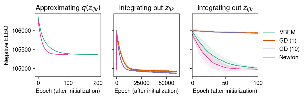
To initialize all methods, run 50 epochs of VBEM. Compare VBEM and Newton-Raphson (which optimize the ELBO eq. 20-21) and gradient descent (which optimizes the ELBO eq. 32). For each method, trace the ELBO estimated according to eq. 32.
# Important: VBEM is randomly initialized
print('fitting initial model by VBEM')
torch.manual_seed(1)
m0 = PMFVBEM(n, p, K).cuda().fit(xt, num_epochs=50, step=1e-3)

models = dict()

# Continue VBEM updates
print('fitting by VBEM')
models['VBEM'] = PMFVBEM(n, p, K).cuda()
models['VBEM'].load_state_dict(m0.state_dict())
models['VBEM'].fit(xt, num_epochs=200, step=1e-3)

# Important: GD is stochastic
print('fitting by GD (1)')
torch.manual_seed(2)
models['GD (1)'] = PMFGD(n, p, K).cuda()
models['GD (1)'].load_state_dict(m0.state_dict())
models['GD (1)'].fit(xt, num_epochs=60000, lr=5e-2, eps=1e-2)

print('fitting by GD (10)')
torch.manual_seed(2)
models['GD (10)'] = PMFGD(n, p, K).cuda()
models['GD (10)'].load_state_dict(m0.state_dict())
models['GD (10)'].fit(xt, num_epochs=60000, n_samples=10, lr=5e-2, eps=1e-2)

print('fitting by Newton-Raphson')
models['Newton'] = PMFN(n, p, K).cuda()
models['Newton'].load_state_dict(m0.state_dict())
models['Newton'].fit(xt, num_epochs=100, step=0.5)
PMFN()
Write out the saved models.
torch.save({k: models[k].state_dict() for k in models},
           '/scratch/midway2/aksarkar/singlecell/hpmf-sim-ex.pt')
Look at the ELBO achieved by the algorithms.
cm = plt.get_cmap('Dark2')
plt.clf()
fig, ax = plt.subplots(1, 3, sharey=True)
fig.set_size_inches(7.5, 2.5)
for i, name in enumerate(models):
  temp = getattr(models[name], 'trace2', None)
  if temp:
    ax[0].plot(temp, c=cm(i), lw=1, marker=None, label=name)
ax[0].set_title('Approximating $q(z_{ijk})$')

for i, name in enumerate(models):
  mu = pd.Series(models[name].trace).ewm(alpha=0.1).mean()
  sd = pd.Series(models[name].trace).ewm(alpha=0.1).std()
  for a in ax[1:]:
    a.plot(mu, c=cm(i), lw=1, marker=None, label=name)
    a.fill_between(np.arange(len(mu)), mu - sd, mu + sd, color=cm(i), alpha=0.1)
    a.set_title('Integrating out $z_{ijk}$')
ax[-1].set_xlim(0, 100)
ax[-1].legend(frameon=False, loc='center left', bbox_to_anchor=(1, .5))
for a in ax:
  a.set_xlabel('Epoch (after initialization)')
ax[0].set_ylabel('Negative ELBO')
fig.tight_layout()
Report the final (approximate) ELBO.
{name: np.array(models[name].trace[-10:]).mean()
 for name in models}
{'VBEM': 104990.25,
'GD (1)': 104915.23,
'GD (10)': 104877.33,
'Newton': 104974.35}
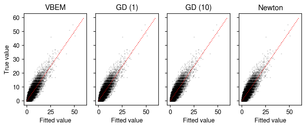
Compare the fitted values of each approach to the observed values.
plt.clf()
fig, ax = plt.subplots(1, 4, sharey=True)
fig.set_size_inches(7, 3)

for a, name in zip(ax, models):
  with torch.no_grad():
    pm = ((models[name].alpha_l / models[name].beta_l) @
          (models[name].alpha_f / models[name].beta_f).T).cpu()
  a.scatter(pm.ravel(), x.ravel(), s=1, alpha=0.1, c='k')
lim = [0, 60]
for a, name in zip(ax, models):
  a.plot(lim, lim, c='r', lw=1, ls=':')
  a.set_xlabel('Fitted value')
  a.set_title(name)
ax[0].set_ylabel('True value')
fig.tight_layout()
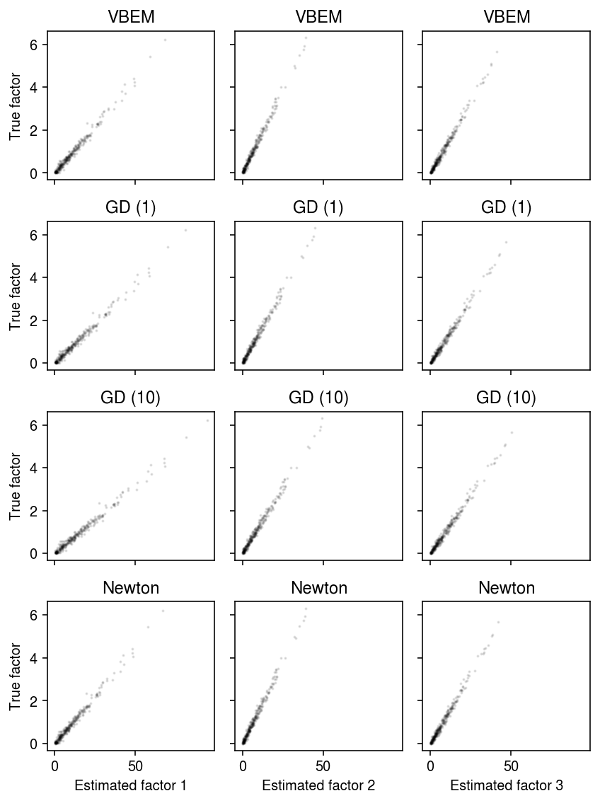
Compare the estimated factors to the ground truth.
plt.clf()
fig, ax = plt.subplots(4, 3, sharex=True, sharey=True)
fig.set_size_inches(6, 8)
for i, (row, name) in enumerate(zip(ax, models)):
  with torch.no_grad():
    pm = (models[name].alpha_f / models[name].beta_f).cpu().numpy()
  order = np.argmax(np.corrcoef(f, pm, rowvar=False)[K:,:K], axis=0)
  for k, a in enumerate(row):
    a.scatter(pm[:,order[k]], f[:,k], s=1, c='k', alpha=0.1)
    a.set_title(name)
  row[0].set_ylabel(f'True factor')
for k, a in enumerate(ax.T):
  a[-1].set_xlabel(f'Estimated factor {k + 1}')
fig.tight_layout()
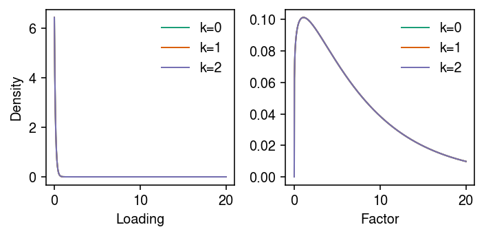
Look at the estimated priors.
cm = plt.get_cmap('Dark2')
plt.clf()
fig, ax = plt.subplots(1, 2)
fig.set_size_inches(5, 2.5)
grid = np.linspace(0, 20, 1000)
for a, k in zip(ax, ('l', 'f')):
  with torch.no_grad():
    g = st.gamma(a=getattr(models['VBEM'], f'a_{k}').cpu()[0,j],
                 scale=1 / getattr(models['VBEM'], f'b_{k}').cpu()[0,j])
  for j in range(K):
    a.plot(grid, g.pdf(grid), lw=1, c=cm(j), label=f'k={j}')
  a.legend(frameon=False)
ax[0].set_ylabel('Density')
ax[0].set_xlabel('Loading')
ax[1].set_xlabel('Factor')
fig.tight_layout()
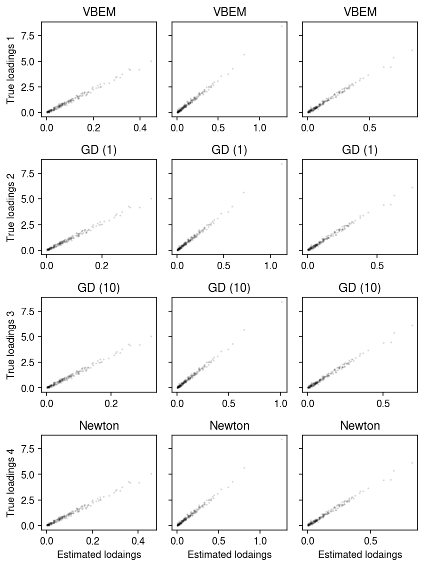
Compare the estimated loadings to the true loadings.
plt.clf()
fig, ax = plt.subplots(4, 3, sharey=True, sharex=False)
fig.set_size_inches(6, 8)
for i, (row, name) in enumerate(zip(ax, models)):
  with torch.no_grad():
    pm = (models[name].alpha_l / models[name].beta_l).cpu().numpy()
  order = np.argmax(np.corrcoef(l, pm, rowvar=False)[K:,:K], axis=0)
  for k, a in enumerate(row):
    a.scatter(pm[:,order[k]], l[:,k], s=1, c='k', alpha=0.1)
    a.set_title(name)
  row[0].set_ylabel(f'True loadings {i+1}')
for a in ax.T:
  a[-1].set_xlabel('Estimated lodaings')
fig.tight_layout()
Correlated factors example
Simulate factors that are correlated by drawing from a log multivariate Gaussian.
rng = np.random.default_rng(1)
n = 200
p = 300
K = 3
a_l = 1
b_l = 1
l = rng.gamma(a_l, b_l, size=(n, K))
cov = np.eye(K)
cov[1,2] = cov[2,1] = 0.6
f = np.exp(rng.multivariate_normal(mean=np.zeros(K), cov=cov, size=(p,)))
x = rng.poisson(l @ f.T)
xt = torch.tensor(x, dtype=torch.float, device='cuda')
To initialize all methods, run 50 epochs of VBEM. Compare VBEM, Newton-Raphson, and gradient descent, tracing the ELBO estimated according to eq. 32.
# Important: VBEM is randomly initialized
print('fitting initial model by VBEM')
torch.manual_seed(1)
m0 = PMFVBEM(n, p, K).cuda().fit(xt, num_epochs=50, step=1e-3)

models = dict()

# Continue VBEM updates
print('fitting by VBEM')
models['VBEM'] = PMFVBEM(n, p, K).cuda()
models['VBEM'].load_state_dict(m0.state_dict())
models['VBEM'].fit(xt, num_epochs=1000, step=1e-3)

# Important: GD is stochastic
print('fitting by GD')
torch.manual_seed(2)
models['GD'] = PMFGD(n, p, K).cuda()
models['GD'].load_state_dict(m0.state_dict())
models['GD'].fit(xt, num_epochs=60000, lr=5e-2, eps=1e-2)

print('fitting by Newton-Raphson')
models['Newton'] = PMFN(n, p, K).cuda()
models['Newton'].load_state_dict(m0.state_dict())
models['Newton'].fit(xt, num_epochs=200, step=0.5)
PMFN()
Look at the ELBO achieved by the algorithms.
cm = plt.get_cmap('Dark2')
plt.clf()
fig, ax = plt.subplots(1, 3)
fig.set_size_inches(7.5, 2.5)
for i, name in enumerate(models):
  temp = getattr(models[name], 'trace2', None)
  if temp:
    ax[0].plot(temp, c=cm(i), lw=1, marker=None, label=name)
ax[0].set_title('Approximating $q(z_{ijk})$')

for i, name in enumerate(models):
  mu = pd.Series(models[name].trace).ewm(alpha=0.1).mean()
  sd = pd.Series(models[name].trace).ewm(alpha=0.1).std()
  for a in ax[1:]:
    a.plot(mu, c=cm(i), lw=1, marker=None, label=name)
    a.fill_between(np.arange(len(mu)), mu - sd, mu + sd, color=cm(i), alpha=0.1)
    a.set_title('Integrating out $z_{ijk}$')
ax[-1].set_xlim(0, 1000)
ax[-1].legend(frameon=False, loc='center left', bbox_to_anchor=(1, .5))
for a in ax:
  a.set_xlabel('Epoch (after initialization)')
ax[0].set_ylabel('Negative ELBO')
fig.tight_layout()
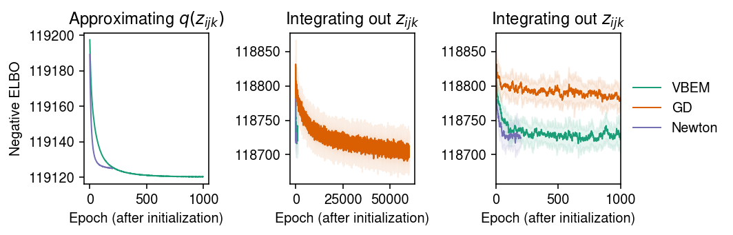
Report the final (approximate) ELBO.
{name: np.array(models[name].trace[-10:]).mean()
 for name in models}
{'VBEM': 118721.9, 'GD': 118704.336, 'Newton': 118723.39}
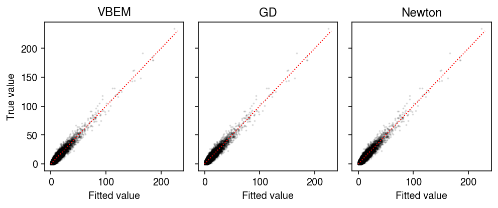
Compare the fitted values of each approach to the observed values.
plt.clf()
fig, ax = plt.subplots(1, 3, sharey=True)
fig.set_size_inches(7, 3)

for a, name in zip(ax, models):
  with torch.no_grad():
    pm = ((models[name].alpha_l / models[name].beta_l) @
          (models[name].alpha_f / models[name].beta_f).T).cpu()
  a.scatter(pm.ravel(), x.ravel(), s=1, alpha=0.1, c='k')
lim = [0, 230]
for a, name in zip(ax, models):
  a.plot(lim, lim, c='r', lw=1, ls=':')
  a.set_xlabel('Fitted value')
  a.set_title(name)
ax[0].set_ylabel('True value')
fig.tight_layout()
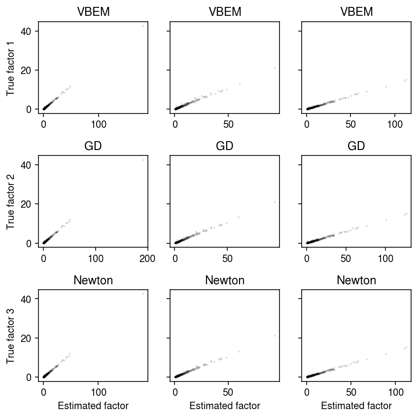
Compare the estimated factors to the ground truth.
plt.clf()
fig, ax = plt.subplots(3, 3, sharey=True, sharex=False)
fig.set_size_inches(6, 6)
for i, (row, name) in enumerate(zip(ax, models)):
  with torch.no_grad():
    pm = (models[name].alpha_f / models[name].beta_f).cpu().numpy()
  order = np.argmax(np.corrcoef(f, pm, rowvar=False)[K:,:K], axis=0)
  for k, a in enumerate(row):
    a.scatter(pm[:,order[k]], f[:,k], s=1, c='k', alpha=0.1)
    a.set_title(name)
  row[0].set_ylabel(f'True factor {i+1}')
for a in ax.T:
  a[-1].set_xlabel('Estimated factor')
fig.tight_layout()
fastTopics example
Peter Carbonetto demonstrated that EM for NMF can fail to make progress, with consequences on e.g., VBEM for LDA.
names = rpy2.robjects.r['load']('/scratch/midway2/aksarkar/singlecell/smallsimb.RData')
dat = {name: rpy2.robjects.r[name] for name in names}
n, p = dat['X'].shape
_, K = dat['L0'].shape
xt = torch.tensor(dat['X'], dtype=torch.float, device='cuda')
Initialize \(\alpha_{lik}, \alpha_{fjk}\) at the given initialization \(\ml_0, \mf_0\) and fix \(\beta_{lk} = 1, \beta_{fk} = 1\).
m0 = PMFVBEM(n, p, K).cuda()
eps = 0.1
m0.alpha_l.data = torch.clamp(torch.tensor(dat['L0']), min=eps)
m0.beta_l.data = torch.ones([1, K])
m0.alpha_f.data = torch.clamp(torch.tensor(dat['F0']), min=eps)
m0.beta_l.data = torch.ones([1, K])
models = dict()
print('fitting by VBEM')
models['VBEM'] = PMFVBEM(n, p, K).cuda()
models['VBEM'].load_state_dict(m0.state_dict())
models['VBEM'].fit(xt, num_epochs=500, step=1e-3)
PMFVBEM()
print('fitting by Newton-Raphson')
models['Newton'] = PMFN(n, p, K).cuda()
models['Newton'].load_state_dict(m0.state_dict())
models['Newton'].fit(xt, num_epochs=50, step=1e-6)
PMFN()
print(f'fitting by GD')
# Important: GD is stochastic
torch.manual_seed(2)
models['GD'] = PMFGD(n, p, K).cuda()
models['GD'].load_state_dict(m0.state_dict())
models['GD'].fit(xt, num_epochs=60000, n_samples=n_samples, lr=1e-4, eps=1e-2)
PMFGD()
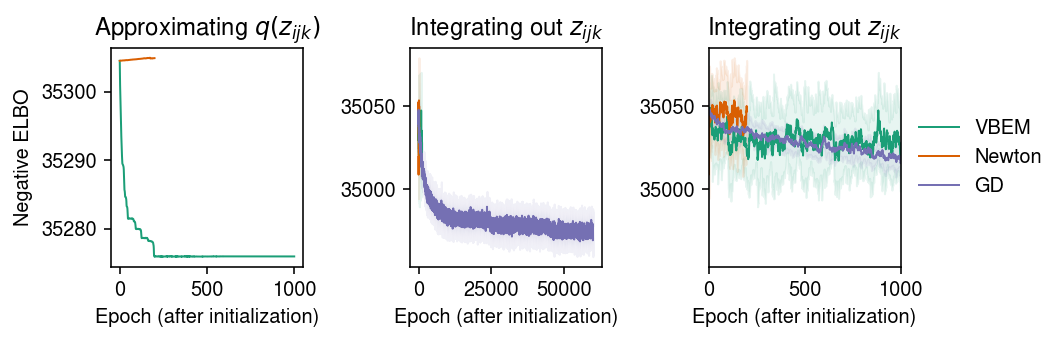
Look at the ELBO achieved by the algorithms.
cm = plt.get_cmap('Dark2')
plt.clf()
fig, ax = plt.subplots(1, 3)
fig.set_size_inches(7.5, 2.5)
for i, name in enumerate(models):
  temp = getattr(models[name], 'trace2', None)
  if temp:
    ax[0].plot(temp, c=cm(i), lw=1, marker=None, label=name)
ax[0].set_title('Approximating $q(z_{ijk})$')

for i, name in enumerate(models):
  mu = pd.Series(models[name].trace).ewm(alpha=0.1).mean()
  sd = pd.Series(models[name].trace).ewm(alpha=0.1).std()
  for a in ax[1:]:
    a.plot(mu, c=cm(i), lw=1, marker=None, label=name)
    a.fill_between(np.arange(len(mu)), mu - sd, mu + sd, color=cm(i), alpha=0.1)
    a.set_title('Integrating out $z_{ijk}$')
ax[-1].set_xlim(0, 500)
ax[-1].legend(frameon=False, loc='center left', bbox_to_anchor=(1, .5))
for a in ax:
  a.set_xlabel('Epoch (after initialization)')
ax[0].set_ylabel('Negative ELBO')
fig.tight_layout()
Report the final (approximate) ELBO.
{name: np.array(models[name].trace[-10:]).mean()
 for name in models}
{'VBEM': 42475.727, 'Newton': 139408.52, 'GD': 63879.742}
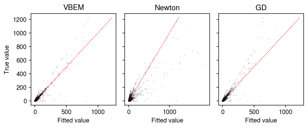
Compare the fitted values of each approach to the observed values.
plt.clf()
fig, ax = plt.subplots(1, 3, sharey=True)
fig.set_size_inches(7, 3)

for a, name in zip(ax, models):
  with torch.no_grad():
    pm = ((models[name].alpha_l / models[name].beta_l) @
          (models[name].alpha_f / models[name].beta_f).T).cpu()
  a.scatter(pm.ravel(), dat['X'].ravel(), s=1, alpha=0.1, c='k')
lim = [0, 1225]
for a, name in zip(ax, models):
  a.plot(lim, lim, c='r', lw=1, ls=':')
  a.set_xlabel('Fitted value')
  a.set_title(name)
ax[0].set_ylabel('True value')
fig.tight_layout()
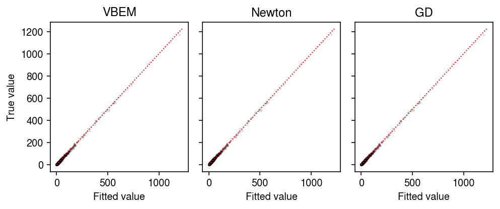
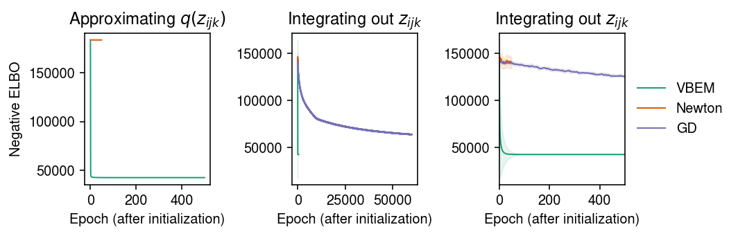
As an alternative initialization, run 50 epochs of VBEM. Compare VBEM, Newton-Raphson, and gradient descent, tracing the ELBO estimated according to eq. 32.
# Important: VBEM is randomly initialized
print('fitting initial model by VBEM')
torch.manual_seed(1)
m0 = PMFVBEM(n, p, K).cuda().fit(xt, num_epochs=50, step=1e-3)

models = dict()

# Continue VBEM updates
print('fitting by VBEM')
models['VBEM'] = PMFVBEM(n, p, K).cuda()
models['VBEM'].load_state_dict(m0.state_dict())
models['VBEM'].fit(xt, num_epochs=1000, step=1e-3)

print('fitting by Newton-Raphson')
models['Newton'] = PMFN(n, p, K).cuda()
models['Newton'].load_state_dict(m0.state_dict())
models['Newton'].fit(xt, num_epochs=200, step=1e-3)

# Important: GD is stochastic
print('fitting by GD')
torch.manual_seed(2)
models['GD'] = PMFGD(n, p, K).cuda()
models['GD'].load_state_dict(m0.state_dict())
models['GD'].fit(xt, num_epochs=60000, n_samples=10, lr=1e-3, eps=1e-2)
PMFGD()
Look at the ELBO achieved by the algorithms.
cm = plt.get_cmap('Dark2')
plt.clf()
fig, ax = plt.subplots(1, 3)
fig.set_size_inches(7.5, 2.5)
for i, name in enumerate(models):
  temp = getattr(models[name], 'trace2', None)
  if temp:
    ax[0].plot(temp, c=cm(i), lw=1, marker=None, label=name)
ax[0].set_title('Approximating $q(z_{ijk})$')

for i, name in enumerate(models):
  mu = pd.Series(models[name].trace).ewm(alpha=0.1).mean()
  sd = pd.Series(models[name].trace).ewm(alpha=0.1).std()
  for a in ax[1:]:
    a.plot(mu, c=cm(i), lw=1, marker=None, label=name)
    a.fill_between(np.arange(len(mu)), mu - sd, mu + sd, color=cm(i), alpha=0.1)
    a.set_title('Integrating out $z_{ijk}$')
ax[-1].set_xlim(0, 1000)
ax[-1].legend(frameon=False, loc='center left', bbox_to_anchor=(1, .5))
for a in ax:
  a.set_xlabel('Epoch (after initialization)')
ax[0].set_ylabel('Negative ELBO')
fig.tight_layout()
Report the final (approximate) ELBO.
{name: np.array(models[name].trace[-10:]).mean()
 for name in models}
{'VBEM': 35019.47, 'Newton': 35052.777, 'GD': 34970.6}
Compare the fitted values of each approach to the observed values.
plt.clf()
fig, ax = plt.subplots(1, 3, sharey=True)
fig.set_size_inches(7, 3)

for a, name in zip(ax, models):
  with torch.no_grad():
    pm = ((models[name].alpha_l / models[name].beta_l) @
          (models[name].alpha_f / models[name].beta_f).T).cpu()
  a.scatter(pm.ravel(), dat['X'].ravel(), s=1, alpha=0.1, c='k')
lim = [0, 1225]
for a, name in zip(ax, models):
  a.plot(lim, lim, c='r', lw=1, ls=':')
  a.set_xlabel('Fitted value')
  a.set_title(name)
ax[0].set_ylabel('True value')
fig.tight_layout()