Empirical Bayes inference for the horseshoe prior

Introduction
Setup
Results
Notes

Introduction

The horseshoe prior (Carvalho et al. 2009) is \( \DeclareMathOperator\N{\mathcal{N}} \DeclareMathOperator\HalfCauchy{C^+} \)

\begin{align} \beta_j \mid \lambda_j, \tau &\sim \N(0, \lambda_j^2 \tau^2)\\ \lambda_j &\sim \HalfCauchy(0, 1). \end{align}

Commonly, it is used as a prior for EBNM

\begin{equation} x_j \mid \beta_j, \sigma^2 \sim \N(\beta_j, \sigma^2). \end{equation}

Inference is commonly performed by MCMC or by VI (e.g. Ghosh and Doshi-Velez 2018); however, recently a fast scheme for EB inference was proposed (van der Pas et al. 2014). Jason Willwerscheid gave an example where EB inference does poorly, which we investigate here.

Setup

import contextlib
import functools as ft
import numpy as np
import pandas as pd
import pyro
import sys
import torch

import rpy2.robjects.packages
import rpy2.robjects.pandas2ri
rpy2.robjects.pandas2ri.activate()
horseshoe = rpy2.robjects.packages.importr('horseshoe')

%matplotlib inline
%config InlineBackend.figure_formats = set(['retina'])

import matplotlib.pyplot as plt
plt.rcParams['figure.facecolor'] = 'w'
plt.rcParams['font.family'] = 'Nimbus Sans'

Results

Simulation

def simulate(n, s, tau, seed):
  rng = np.random.default_rng(seed)
  lam = abs(rng.standard_cauchy(size=n))
  beta = rng.normal(scale=s * lam * tau)
  x = rng.normal(loc=beta, scale=s)
  return x, beta

def _ebnm_horseshoe(x, s, tauhat):
  lam = pyro.sample('lam', pyro.distributions.HalfCauchy(scale=torch.ones(x.shape[0])))
  b = pyro.sample('b', pyro.distributions.Normal(loc=torch.zeros(x.shape[0]), scale=1.))
  beta = lam * b * tauhat
  return pyro.sample('x', pyro.distributions.Normal(loc=beta, scale=s), obs=x)

def run_nuts(x, s, tauhat, num_samples=100, warmup_steps=100, verbose=True, **kwargs):
  nuts = pyro.infer.mcmc.NUTS(_ebnm_horseshoe)
  samples = pyro.infer.mcmc.MCMC(nuts, num_samples=num_samples, warmup_steps=warmup_steps)
  samples.run(torch.tensor(x), torch.tensor(s), torch.tensor(tauhat))
  return (tauhat * samples.get_samples()['b'] * samples.get_samples()['lam']).mean(dim=0).numpy()

def run_mcmc(x, s, tauhat, burn=1000, **kwargs):
  with contextlib.redirect_stdout(None):
    pm = horseshoe.HS_normal_means(x, method_tau='fixed', tau=tauhat,
                                   method_sigma='fixed', Sigma2=s ** 2,
                                   burn=burn).rx2('BetaHat')
  return pm

def run_analytic(x, s, tauhat, **kwargs):
  try:
    pm = horseshoe.HS_post_mean(x, tauhat, s ** 2)
  except:
    pm = np.full(np.nan, beta.shape)
  return pm

def mse(betahat, beta):
  return np.square(betahat - beta).mean()

def trial(n, s, tau, seed=1, methods=['mcmc', 'analytic'], **kwargs):
  x, beta = simulate(n, s, tau, seed)
  tauhat = horseshoe.HS_MMLE(x, s ** 2)[0]
  res = {f'mse_{m}': mse(globals()[f'run_{m}'](x, s, tauhat, **kwargs), beta)
         for m in methods}
  res['n'] = n
  res['s'] = s
  res['tau'] = tau
  res['tauhat'] = tauhat
  res['trial'] = seed
  return pd.Series(res)

def evaluate(s, tau, n_trials=1, **kwargs):
  res = []
  for n in (100, 500, 1000):
    for i in range(n_trials):
      res.append(trial(n, s, tau, seed=i, **kwargs))
  return pd.DataFrame(res)

Scenario 1

Use the hyperparameters Jason used.

s = 2
tau = 0.3
x, beta = simulate(n=100, s=s, tau=tau, seed=3)
tauhat = horseshoe.HS_MMLE(x, s ** 2)[0]
pm_mcmc = run_mcmc(x, s=s, tauhat=tauhat)
pm_analytic = run_analytic(x, s=s, tauhat=tauhat)
pm_nuts = run_nuts(x, s=s, tauhat=tauhat)

Compare the estimated posterior means by MCMC vs. the analytic solution.

plt.clf()
fig, ax = plt.subplots(1, 3, sharey=True)
fig.set_size_inches(5.5, 2.5)

for a in ax:
  a.set_aspect('equal', adjustable='datalim')

ax[0].scatter(pm_mcmc, beta, c='k', s=4)
ax[0].set_xlabel(r'Estimated $\hat\beta$ (Gibbs)')
ax[0].set_ylabel(r'Simulated $\beta$')

ax[1].scatter(pm_analytic, beta, c='k', s=4)
ax[1].set_xlabel(r'Estimated $\hat\beta$ (analytic)')

ax[2].scatter(pm_nuts, beta, c='k', s=4)
ax[2].set_xlabel(r'Estimated $\hat\beta$ (NUTS)')

fig.tight_layout()

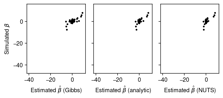
pd.Series({'mcmc': mse(pm_mcmc, beta),
           'nuts': mse(pm_nuts, beta),
           'analytic': mse(pm_analytic, beta)})

mcmc        1.934118
nuts        1.004739
analytic    1.043704
dtype: float64

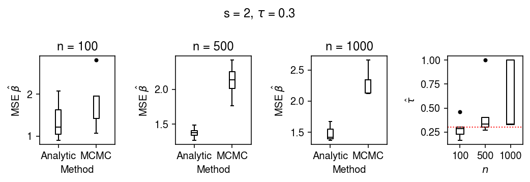
Evaluate how the accuracy of inference depends on random seed and sample size.

res = evaluate(s=2, tau=0.3, n_trials=5)

plt.clf()
fig, ax = plt.subplots(1, 4)
fig.set_size_inches(7.5, 2.5)

for a, n in zip(ax, [100, 500, 1000]):
  query = res[res['n'] == n].pivot_table(index='trial', values=['mse_mcmc', 'mse_analytic']).values
  a.boxplot([np.ma.masked_invalid(q).compressed() for q in query.T],
            medianprops={'color': 'k'}, flierprops={'marker': '.', 'markerfacecolor': 'k'})
  a.set_title(f'n = {n}')
  a.set_xlabel('Method')
  a.set_xticklabels(['Analytic', 'MCMC'])
  a.set_ylabel(r'MSE $\hat\beta$')

ax[-1].boxplot(res.pivot_table(index='trial', columns='n', values='tauhat').values,
               medianprops={'color': 'k'}, flierprops={'marker': '.', 'markerfacecolor': 'k'})
ax[-1].axhline(y=0.3, c='r', ls=':', lw=1)
ax[-1].set_xlabel('$n$')
ax[-1].set_xticklabels([100, 500, 1000])
ax[-1].set_ylabel(r'$\hat{\tau}$')

fig.suptitle(r's = 2, $\tau$ = 0.3')
fig.tight_layout()

sim-s-2-tau-0.3.png

Scenario 2

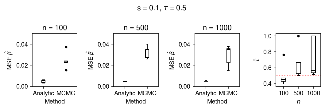
Try a different setting of the hyperparameters.

res = evaluate(s=0.1, tau=0.5, n_trials=5)

plt.clf()
fig, ax = plt.subplots(1, 4)
fig.set_size_inches(7.5, 2.5)

for a, n in zip(ax, [100, 500, 1000]):
  query = res[res['n'] == n].pivot_table(index='trial', values=['mse_mcmc', 'mse_analytic']).values
  a.boxplot([np.ma.masked_invalid(q).compressed() for q in query.T],
            medianprops={'color': 'k'}, flierprops={'marker': '.', 'markerfacecolor': 'k'})
  a.set_title(f'n = {n}')
  a.set_xlabel('Method')
  a.set_xticklabels(['Analytic', 'MCMC'])
  a.set_ylabel(r'MSE $\hat\beta$')
  a.set_ylim(0, 0.05)

ax[-1].boxplot(res.pivot_table(index='trial', columns='n', values='tauhat').values,
               medianprops={'color': 'k'}, flierprops={'marker': '.', 'markerfacecolor': 'k'})
ax[-1].axhline(y=0.5, c='r', ls=':', lw=1)
ax[-1].set_xlabel('$n$')
ax[-1].set_xticklabels([100, 500, 1000])
ax[-1].set_ylabel(r'$\hat{\tau}$')

fig.suptitle(r's = 0.1, $\tau$ = 0.5')
fig.tight_layout()

Find the cases where the analytic solution failed.

res[np.isnan(res['mse_analytic'])]

mse_mcmc  mse_analytic       n    s  tau    tauhat  trial
6   0.027008           NaN   500.0  0.1  0.5  0.999934    1.0
11  0.015194           NaN  1000.0  0.1  0.5  0.999934    1.0
13  0.022354           NaN  1000.0  0.1  0.5  0.999934    3.0

Look at the simulated data for one of the cases.

x, beta = simulate(n=500, s=0.1, tau=0.5, seed=1)

x.min(), beta.min()

(-572.0789680814781, -571.9190274305989)

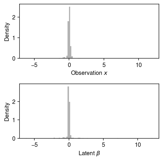
Plot the simulated data, omitting outliers.

plt.clf()
fig, ax = plt.subplots(2, 1)
fig.set_size_inches(4, 4)

ax[0].hist(x[x > -80], bins=100, color='0.7', density=True)
ax[0].set_xlabel('Observation $x$')
ax[0].set_ylabel('Density')

ax[1].hist(beta[beta > -80], bins=100, color='0.7', density=True)
ax[1].set_xlabel(r'Latent $\beta$')
ax[1].set_ylabel('Density')

fig.tight_layout()

Notes

In these simulations, there are surprisingly often very large outlier values of \(\beta\) (and therefore \(x\)), leading to an estimate \(\hat\tau = 1\). These in turn appear to lead to failures in numerically integrating to estimate the marginal likelihood (as a subroutine in derivate-free optimization).

Ghosh and Doshi-Velez 2018 note that the prior exhibits strong correlation between \(\beta_j\) and \(\lambda_j \tau\), which makes MCMC very difficult. Instead, they suggest a non-centered parameterization

\begin{align} \beta_j &= b_j \lambda_j \tau\\ b_j &\sim \N(0, 1)\\ \lambda_j &\sim \HalfCauchy(0, 1), \end{align}

in which the prior is marginally uncorrelated. However, it is not clear that this is the parameterization used in the implementation of horseshoe::HS.normal.means.