Normalizing flows for EBPM
Table of Contents
Introduction
Fitting an expression model to observed scRNA-seq data at a single gene can be thought of as solving an empirical Bayes problem (Sarkar and Stephens 2020). \( \DeclareMathOperator\Pois{Poisson} \DeclareMathOperator\Gam{Gamma} \DeclareMathOperator\E{E} \DeclareMathOperator\V{V} \DeclareMathOperator\N{\mathcal{N}} \newcommand\abs[1]{\left\vert #1 \right\vert} \newcommand\const{\mathrm{const}} \)
\begin{align} x_i \mid s_i, \lambda_i &\sim \Pois(s_i \lambda_i)\\ \lambda_i &\sim g(\cdot) \in \mathcal{G}, \end{align}where \(i = 1, \ldots, n\) indexes samples. Assuming \(\mathcal{G}\) is the family of Gamma distributions yields analytic gradients and admits fast implementation on GPUs. However, the fitted model can fail to accurately describe expression variation at some genes.
In contrast, the family of non-parametric unimodal distributions (Stephens 2017) could be sufficient for all but a minority of genes. In practice, this family is approximated as the family of mixture of uniform distributions with fixed endpoints \(a_k\) and common mode \(\lambda_0\)
\begin{equation} \lambda_i \sim \sum_{k=1}^K \pi_k \operatorname{Uniform}(\lambda_0, a_k). \end{equation}Then, inference in this model can be achieved by a combination of convex optimization (over \(\boldsymbol{\pi}\), given \(\lambda_0\)) and line search (over \(\lambda_0\), as an outer loop). However, in practice this approach is expensive and cumbersome to parallelize for large data sets.
One idea which could bridge the gap between these approaches (in both computational cost and flexibility) is normalizing flows (reviewed in Papamakarios et al. 2019). The key idea of normalizing flows is to apply a series of invertible, differentiable transformations \(T_1, \ldots, T_K\) to a tractable density, in order to obtain a different density. It is sometimes more convenient to instead work with the inverse transformation
\begin{align} u &= (T_K \circ \cdots \circ T_1)(x)\\ f_x(x) &= f_u(u) \prod_{k=1}^{K} \det \abs{J_k(\cdot)}, \end{align}where \(J_k\) is the Jacobian of \(T_k\). If the functions \(T_k\) have free parameters, gradients with respect to those parameters are available, allowing the transformations to be learned from the data. Here, we investigate using flows to define a flexible family of priors, and use that family to fit expression models to scRNA-seq data.
Setup
import anndata
import numpy as np
import pandas as pd
import scipy.integrate as si
import scipy.special as sp
import scipy.stats as st
import scmodes
import torch
import torch.utils.tensorboard as tb
import rpy2.robjects.packages
import rpy2.robjects.pandas2ri
rpy2.robjects.pandas2ri.activate()
ashr = rpy2.robjects.packages.importr('ashr')
%matplotlib inline
%config InlineBackend.figure_formats = set(['svg'])
import colorcet
import matplotlib.pyplot as plt
plt.rcParams['figure.facecolor'] = 'w'
plt.rcParams['font.family'] = 'Nimbus Sans'
Methods
Planar flow
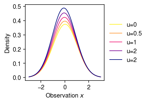
The specific class of transformations we will consider are planar flows (Rezende and Mohamed 2015)
\begin{equation} T(x) = x + u \operatorname{sigmoid}(w x + b), \end{equation}where \(u, w, b\) are free (scalar) parameters.
class PlanarFlow(torch.nn.Module):
  # Rezende and Mohamed 2015
  def __init__(self, n_features, random_init=True):
    super().__init__()
    self.weight = torch.nn.Parameter(torch.zeros([n_features, 1]))
    self.bias = torch.nn.Parameter(torch.zeros([1]))
    self.post_act = torch.nn.Parameter(torch.zeros([n_features, 1]))
    if random_init:
      torch.nn.init.xavier_normal_(self.weight)
      torch.nn.init.xavier_normal_(self.post_act)

  def forward(self, x, eps=1e-15):
    # x is [batch_size, n_features]
    pre_act = x @ self.weight + self.bias
    # This is required to invert the flow
    post_act = self.post_act + self.weight / (self.weight.T @ self.weight + eps) * (-1 + torch.nn.functional.softplus(self.weight.T @ self.post_act) - self.weight.T @ self.post_act)
    out = x + torch.sigmoid(pre_act) @ post_act.T
    log_det = torch.log(torch.abs(1 + torch.sigmoid(pre_act) * torch.sigmoid(-pre_act) @ self.weight.T @ post_act))
    assert not torch.isnan(log_det).any()
    return out, log_det

  def __repr__(self):
    return f'PlanarFlow(post_act={self.post_act.data}, weight={self.weight.data}, bias={self.bias.data})'

# Important: these are needed to transform distributions with constrained
# support to unconstrained support

# y = softplus(x) = log1p(exp(x))

# dy/dx = exp(x) / (1 + exp(x)) = sigmoid(x)

class Softplus(torch.nn.Module):
  def __init__(self):
    super().__init__()

  def forward(self, x):
    return torch.nn.functional.softplus(x), torch.log(torch.sigmoid(x))

# x = softplus^{-1}(y) = ln(expm1(y))

# dx/dy = exp(y) / (exp(y) - 1) = 1 / (1 - exp(-y))

class InverseSoftplus(torch.nn.Module):
  def __init__(self):
    super().__init__()

  def forward(self, x):
    # c.f. https://github.com/tensorflow/probability/blob/v0.12.1/tensorflow_probability/python/math/generic.py#L456-L507
    return torch.log(torch.expm1(x)), x - torch.log(torch.expm1(x))

# For completeness. In preliminary experiments, Exp tends to overflow

class Exp(torch.nn.Module):
  def __init__(self):
    super().__init__()

  def forward(self, x):
    return torch.exp(x), x

class Log(torch.nn.Module):
  def __init__(self):
    super().__init__()

  def forward(self, x):
    assert (x > 0).all()
    return torch.log(x), -torch.log(x)

class NormalizingFlow(torch.nn.Module):
  # https://pytorch.org/docs/stable/_modules/torch/nn/modules/container.html#Sequential
  def __init__(self, flows, use_cuda=True):
    super().__init__()
    self.use_cuda = use_cuda
    self.flows = torch.nn.ModuleList(flows)

  def forward(self, x):
    log_det = torch.zeros(x.shape)
    if torch.cuda.is_available and self.use_cuda:
      log_det = log_det.cuda()
    for f in self.flows:
      x, l = f.forward(x)
      log_det += l
    return x, log_det
The intuition behind this transform is that the pre-activation \(w x + b\) defines a (hyper)plane, and the post-activation \(u\) dilates the density about that hyperplane.
cm = colorcet.cm['bmy']
T = PlanarFlow(1)
T.weight.data = torch.ones([1, 1])
T.bias.data = torch.ones([1, 1])
grid = np.linspace(-3, 3, 1000)

plt.clf()
plt.gcf().set_size_inches(3.5, 2.5)
for u in np.linspace(0, 2, 5):
  T.post_act.data = torch.tensor(np.array(u).reshape(-1, 1), dtype=torch.float)
  with torch.no_grad():
    log_det = T.forward(torch.tensor(grid.reshape(-1, 1), dtype=torch.float))[1].numpy().squeeze()
  plt.plot(grid, np.exp(st.norm().logpdf(grid) + log_det), lw=1, c=cm((2 - u) / 2), label=f'u={u:.1g}')
plt.legend(frameon=False, loc='center left', bbox_to_anchor=(1, .5))
plt.xlabel('Observation $x$')
plt.ylabel('Density')
plt.tight_layout()
Normalizing flow for density estimation
Suppose we have observations \(x_1, \ldots, x_n\) drawn from \(f^*\). One can estimate \(f_x\) by maximizing the likelihood of the data
\begin{align} &\max_{f_x} \E_{f^*}[\ln f_x(x)]\\ = &\max_{T_1, \ldots, T_K} \E_{f^*}\left[\ln f_u(T(x)) + \sum_{k=1}^K \ln\det J_k(\cdot)\right]\\ = &\max_{T_1, \ldots, T_K} \frac{1}{n} \sum_i\left[\ln f_u(T(x_i)) + \sum_{k=1}^K \ln\det J_k(\cdot)\right], \end{align}where \(T = T_K \circ \cdots \circ T_1\) is the mapping from \(x \in \mathcal{X} \rightarrow u \in \mathcal{U}\), and \(f_u\) is the density of some simple distribution (e.g., standard Gaussian). This optimization problem can be readily solved using automatic differentiation and gradient descent.
class DensityEstimator(torch.nn.Module):
  def __init__(self, n_features, K):
    super().__init__()
    # Important: here the flow maps x in ambient measure to u in base measure
    self.flow = NormalizingFlow([PlanarFlow(n_features) for _ in range(K)])

  def forward(self, x):
    loss = -self.log_prob(x).mean()
    assert loss > 0
    return loss

  def fit(self, x, n_epochs, log_dir=None, **kwargs):
    if log_dir is not None:
      writer = tb.SummaryWriter(log_dir)
    opt = torch.optim.RMSprop(self.parameters(), **kwargs)
    global_step = 0
    for _ in range(n_epochs):
      opt.zero_grad()
      loss = self.forward(x)
      if log_dir is not None:
        writer.add_scalar('loss', loss, global_step)
      if torch.isnan(loss):
        raise RuntimeError
      loss.backward()
      opt.step()
      global_step += 1
    return self

  def log_prob(self, x):
    u, log_det = self.flow.forward(x)
    l = torch.distributions.Normal(loc=0., scale=1.).log_prob(u) + log_det
    return l
Normalizing flow for empirical Bayes
Now consider the EBPM problem
\begin{align} x_i \mid s_i, \lambda_i &\sim \Pois(s_i \lambda_i)\\ \lambda_i &\sim g(\cdot) = g_0(\cdot) \prod_k \det \abs{J^g_k} \end{align}where \(i = 1, \ldots, n\), and \(g_0(\cdot) = \N(\cdot; 0, 1)\) for simplicity. One can estimate \(g\) by maximizing the marginal likelihood
\begin{align} &\max_g \sum_i \ln p(x_i \mid s_i, g)\\ \geq &\max_{g, q} \E_{\lambda_i \sim q}\left[\sum_i \ln p(x_i \mid s_i, \lambda_i) + \ln g(\lambda_i) - \ln q(\lambda_i)\right]\\ = &\max_{T_g, q} \E_{\lambda_i \sim q}\left[\sum_i \ln p(x_i \mid s_i, \lambda_i) + \ln g_0(T_g(\lambda_i)) + \sum_k \ln\det\abs{J^g_k} - \ln q(\lambda_i)\right]\\ \end{align}where \(T_g = T^g_K \circ \cdots \circ T^g_1\) maps \(g\) to a base measure and \(J^g_k\) denotes the Jacobian of \(T^g_k\). It is straightforward to show that, holding \(g\) fixed, the optimal \(q\) is the true posterior \(p(\lambda_i \mid x_i, s_i, g)\) (e.g., Neal and Hinton 1998). In order to ensure \(q\) is flexible enough to capture the true posterior, suppose it too is represened by a normalizing flow
\begin{equation} q(\cdot) = q_0(\cdot) \prod_k \det\abs{J^q_k}, \end{equation}where \(J^q_k\) denotes the Jacobian of the transform \(T^q_k\). In order to make sampling easy, suppose \(T_q = T^q_K \circ \cdots \circ T^q_1\) maps the base measure \(q_0(u_i \mid x_i)\) to \(q\). Then, the optimization problem is
\begin{equation} \max_{T_g, T_q} \E_{u_i \sim q_0}\left[\sum_i \ln p(x_i \mid s_i, T_q(u_i)) + \ln g_0(T_g(T_q(u_i))) + \sum_k \ln\det\abs{J^g_k} - \ln q_0(u_i) + \sum_k \ln\det\abs{J^q_k}\right]. \end{equation}Remark It is critical that \(u_i \sim q_0\) depends on \(x_i\) in the variational approximation. Rezende and Mohamed 2015 propose using amortized inference; however, in the context of this problem, a simpler alternative could be a log-Gamma posterior.
Remark Since the transformation \(T_q\) maps \(u_i \in \mathcal{U}\) to \(\lambda_i \in \Lambda\), the signs of the log determinant terms need to be inverted.
Since \(T_g, T_q\) are differentiable, this problem can be solved by replacing the expectation with a Monte Carlo integral (e.g., Kingma and Welling 2014), and then using automatic differentiation and gradient descent to optimize the resulting stochastic objective.
Remark When reducing problems in scRNA-seq data analysis to EBPM, we are primarily interested in the estimated prior \(\hat{g}\). Depending on the choice of flow, obtaining expectations with respect to \(\hat{g}\) might be difficult. One possibility is to approximate these expectations by discretizing \(\hat{g}\) and taking weighted sums.
class EBNM(torch.nn.Module):
  def __init__(self, K, scale, random_init=True, use_cuda=False):
    super().__init__()
    self.scale = scale
    self.p0 = torch.distributions.Normal(loc=0., scale=1.)
    self.pz = NormalizingFlow([PlanarFlow(n_features=1, random_init=random_init) for _ in range(K)], use_cuda=use_cuda)
    self.qz = NormalizingFlow([PlanarFlow(n_features=1, random_init=random_init) for _ in range(K)], use_cuda=use_cuda)

  def forward(self, x, n_samples):
    q0 = torch.distributions.Normal(
      loc=x / (1 + self.scale ** 2),
      scale=torch.sqrt(1 / (1 + 1 / self.scale ** 2)))
    u = q0.rsample(n_samples)
    z, log_det_q = self.qz.forward(u)
    w, log_det_p = self.pz.forward(z)
    # Important: qz is forward transforms, so we need to invert the sign of
    # log_det_q
    elbo = (torch.distributions.Normal(z, self.scale).log_prob(x)
            + self.p0.log_prob(w) + log_det_p
            - (q0.log_prob(u) - log_det_q)).mean(dim=0).sum()
    assert elbo <= 0
    return -elbo

  def fit(self, x, n_epochs, n_samples=1, log_dir=None, **kwargs):
    if log_dir is not None:
      writer = tb.SummaryWriter(log_dir)
    n_samples = torch.Size([n_samples])
    opt = torch.optim.RMSprop(self.parameters(), **kwargs)
    global_step = 0
    for _ in range(n_epochs):
      opt.zero_grad()
      loss = self.forward(x, n_samples)
      if log_dir is not None:
        writer.add_scalar('loss', loss, global_step)
      if torch.isnan(loss):
        raise RuntimeError
      loss.backward()
      opt.step()
      global_step += 1
    return self

  @torch.no_grad()
  def fitted_g(self, z, log=True):
    u, log_det = self.pz.forward(z)
    log_prob = self.p0.log_prob(u) + log_det
    if log:
      return log_prob.numpy()
    else:
      return torch.exp(log_prob).numpy()
class EBPM(torch.nn.Module):
  def __init__(self, K, a=1., b=1.):
    super().__init__()
    self.p0 = torch.distributions.Gamma(concentration=torch.tensor(a, device='cuda', dtype=torch.float),
                                        rate=torch.tensor(b, device='cuda', dtype=torch.float))
    self.pz = NormalizingFlow([InverseSoftplus()] + [PlanarFlow(1) for _ in range(K)] + [Softplus()])
    self.qz = NormalizingFlow([InverseSoftplus()] + [PlanarFlow(1) for _ in range(K)] + [Softplus()])

  def forward(self, x, s, weighted, n_samples):
    q0 = torch.distributions.Gamma(concentration=self.p0.concentration + x, rate=self.p0.rate + s)
    u = q0.rsample(n_samples)
    z, log_det_q = self.qz.forward(u)
    w, log_det_p = self.pz.forward(z)
    log_weights = (torch.distributions.Poisson(s * z).log_prob(x)
                   + self.p0.log_prob(w) + log_det_p
                   - (q0.log_prob(u) - log_det_q))
    if weighted:
      norm_weights = torch.softmax(log_weights, dim=0)
      elbo = (norm_weights * log_weights).sum()
    else:
      elbo = log_weights.mean(dim=0).sum()
    assert elbo <= 0
    return -elbo

  def fit(self, x, s, n_epochs, weighted=False, n_samples=1, log_dir=None, **kwargs):
    if torch.cuda.is_available:
      self.cuda()
    if log_dir is not None:
      writer = tb.SummaryWriter(log_dir)
    n_samples = torch.Size([n_samples])
    opt = torch.optim.RMSprop(self.parameters(), **kwargs)
    global_step = 0
    for _ in range(n_epochs):
      opt.zero_grad()
      loss = self.forward(x, s, weighted=weighted, n_samples=n_samples)
      if log_dir is not None:
        writer.add_scalar('loss', loss, global_step)
      if torch.isnan(loss):
        raise RuntimeError
      loss.backward()
      opt.step()
      global_step += 1
    return self

  @torch.no_grad()
  def fitted_g(self, z, log=True):
    u, log_det = self.pz.forward(z)
    log_prob = self.p0.log_prob(u) + log_det
    if torch.cuda.is_available:
      log_prob = log_prob.cpu()
    if log:
      return log_prob.numpy()
    else:
      return torch.exp(log_prob).numpy()
Results
Example of density estimation
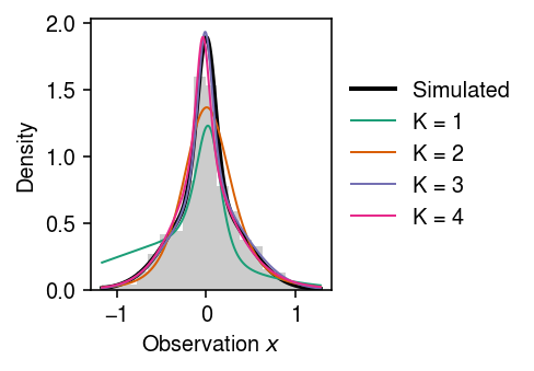
Draw data from a scale mixture of Gaussians.
rng = np.random.default_rng(1)
n = 1000
pi = np.array([0.3, 0.7])
scale = np.array([0.1, 0.4])
z = rng.uniform(size=(n, 1)) < pi[0]
x = rng.normal(scale=scale @ np.hstack([z, ~z]).T)
Fit normalizing flows for different choices of \(K\).
run = 0
lr = 1e-2
n_epochs = 8000
torch.manual_seed(run)
models = [DensityEstimator(n_features=1, K=K)
          .fit(torch.tensor(x.reshape(-1, 1), dtype=torch.float),
               n_epochs=n_epochs,
               lr=lr) for K in range(1, 5)]
Plot the fit.
cm = plt.get_cmap('Dark2')
plt.clf()
plt.gcf().set_size_inches(3.5, 2.5)
plt.hist(x, bins=19, density=True, color='0.8')
grid = np.linspace(x.min(), x.max(), 5000)
mixpdf = st.norm(scale=scale).pdf(grid.reshape(-1, 1)) @ pi
plt.plot(grid, mixpdf, lw=2, c='k', label='Simulated')
for k, m in enumerate(models):
  with torch.no_grad():
    f = np.exp(m.log_prob(torch.tensor(grid.reshape(-1, 1), dtype=torch.float)).numpy())
  plt.plot(grid, f, lw=1, c=cm(k), label=f'K = {k + 1}')
plt.legend(frameon=False, loc='center left', bbox_to_anchor=(1, .5))
plt.xlabel('Observation $x$')
plt.ylabel('Density')
plt.tight_layout()
Density estimation sanity check
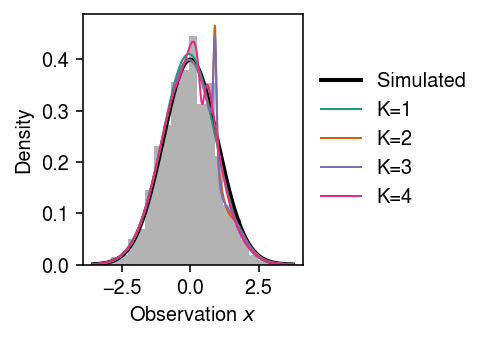
Make sure the method can learn the identity transform. Draw data from a standard Gaussian.
rng = np.random.default_rng(1)
n = 1000
x = rng.normal(size=n)
Fit the model.
run = 0
lr = 1e-2
n_epochs = 8000
torch.manual_seed(run)
models = [DensityEstimator(n_features=1, K=K)
          .fit(torch.tensor(x.reshape(-1, 1), dtype=torch.float),
               n_epochs=n_epochs,
               lr=lr) for K in range(1, 5)]
Plot the fitted models against the simulated data.
cm = plt.get_cmap('Dark2')
plt.clf()
plt.gcf().set_size_inches(3.5, 2.5)
plt.hist(x, bins=23, density=True, color='0.7')
grid = np.linspace(x.min(), x.max(), 1000)
plt.plot(grid, st.norm().pdf(grid), lw=2, c='k', label='Simulated')
for k, m in enumerate(models):
  with torch.no_grad():
    flow = np.exp(m.log_prob(torch.tensor(grid.reshape(-1, 1), dtype=torch.float)).numpy())
  plt.plot(grid, flow, lw=1, c=cm(k), label=f'K={k + 1}')
plt.legend(frameon=False, loc='center left', bbox_to_anchor=(1, .5))
plt.xlabel('Observation $x$')
plt.ylabel('Density')
plt.tight_layout()
EBNM via VBEM sanity check
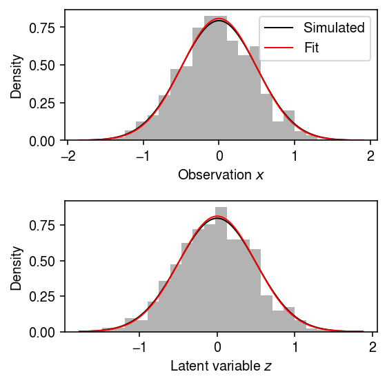
A critical assumption we make is that optimizing the ELBO will yield the correct \(\hat{g}\) if the space of approximations \(q \in \mathcal{Q}\) contains the true posterior. The intuition behind this assumption is that, in this case, VBEM equals EM (Neal and Hinton 1998). Check whether this is the case for a simple example
\begin{align} x_i \mid z_i, s_i^2 &\sim \N(z_i, s_i^2), \qquad i = 1, \ldots, n\\ z_i &\sim \N(0, \sigma_0^2). \end{align}The exact posterior
\begin{align} q(z_i \mid x_i, s_i^2, \sigma_0^2) &= \N\left(\frac{\sigma_0^2}{\sigma_0^2 + s_i^2} x_i, \frac{1}{1 / \sigma_0^2 + 1 / s_i^2}\right)\\ &\triangleq \N(\mu_i, \sigma_i^2) \end{align}and the ELBO is
\begin{align} h &\triangleq \E\left[\sum_i \ln p(x_i, z_i \mid s_i^2, \sigma_0^2) - \ln q(z_i \mid x_i, s_i^2, \sigma_0^2)\right]\\ &= \sum_i -\ln s_i^2 - \frac{(x_i - \E[z_i])^2 - \V[z_i]}{2 s_i^2} - \ln \sigma_0^2 - \frac{\E[z_i]^2 - \V[z_i]}{2 \sigma_0^2} - \ln \sigma_i^2 + \const, \end{align}where expectations are with respect to \(q\), yielding M step update
\begin{align} \frac{\partial h}{\partial \sigma_0^2} &= \frac{n}{\sigma_0^2} - \frac{1}{(\sigma_0^2)^2} \sum_i \E[z_i]^2 - \V[z_i] = 0\\ \sigma_0^2 &:= \frac{1}{n} \sum_i \E[z_i]^2 - \V[z_i] \end{align}def ebnm_em(x, s2, max_iters=100, tol=1e-3): init = np.array([1]) sigma2hat, elbo = squarem(init, _ebnm_elbo, _ebnm_update, x=x, s2=s2, max_iters=max_iters, tol=tol) return sigma2hat, elbo def _ebnm_elbo(sigma2, x, s2): pm = sigma2 / (sigma2 + s2) * x pv = 1 / (1 / sigma2 + 1 / s2) return (-np.log(s2) - ((x - pm) ** 2 - pv) / (2 * s2) - np.log(sigma2) - (pm ** 2 - pv) / (2 * sigma2)).sum() def _ebnm_update(sigma2, x, s2): pm = sigma2 / (sigma2 + s2) * x pv = 1 / (1 / sigma2 + 1 / s2) sigma2 = (pm ** 2 - pv).mean() assert sigma2 >= 0 return sigma2 def squarem(init, objective_fn, update_fn, max_iters, tol, par_tol=1e-8, max_step_updates=10, *args, **kwargs): """Squared extrapolation scheme for accelerated EM Reference: Varadhan, R. and Roland, C. (2008), Simple and Globally Convergent Methods for Accelerating the Convergence of Any EM Algorithm. Scandinavian Journal of Statistics, 35: 335-353. doi:10.1111/j.1467-9469.2007.00585.x """ theta = init obj = objective_fn(theta, *args, **kwargs) for i in range(max_iters): x1 = update_fn(theta, *args, **kwargs) r = x1 - theta if i == 0 and objective_fn(x1, *args, **kwargs) < obj: # Hack: this is needed for numerical reasons, because in e.g., # ebpm_gamma, a point mass is the limit as a = 1/φ → ∞ return init, obj x2 = update_fn(x1, *args, **kwargs) v = (x2 - x1) - r if np.linalg.norm(v) < par_tol: return x2, objective_fn(x2, *args, **kwargs) step = -np.sqrt(r @ r) / np.sqrt(v @ v) if step > -1: step = -1 theta += -2 * step * r + step * step * v update = objective_fn(theta, *args, **kwargs) diff = update - obj else: # Step length = -1 is EM; use as large a step length as is feasible to # maintain monotonicity for j in range(max_step_updates): candidate = theta - 2 * step * r + step * step * v update = objective_fn(candidate, *args, **kwargs) diff = update - obj if np.isfinite(update) and diff > 0: theta = candidate break else: step = (step - 1) / 2 else: step = -1 theta += -2 * step * r + step * step * v update = objective_fn(theta, *args, **kwargs) diff = update - obj if diff < tol: return theta, update else: obj = update else: raise RuntimeError(f'failed to converge in max_iters ({diff:.3g} > {tol:.3g})')
Draw from the model.
rng = np.random.default_rng(1)
n = 1000
s = 0.05
sigma = 0.5
mu = rng.normal(scale=sigma, size=n)
x = rng.normal(loc=mu, scale=s)
Fit VBEM.
sigma2hat, trace = ebnm_vbem(x, s ** 2, max_iters=1000)
Plot the simulated data and model fit.
plt.clf()
fig, ax = plt.subplots(2, 1)
fig.set_size_inches(4, 4)
ax[0].hist(x, bins=25, density='True', color='0.7')
grid = np.linspace(x.min(), x.max(), 1000)
ax[0].plot(grid, st.norm(scale=np.sqrt(s ** 2 + sigma ** 2)).pdf(grid), lw=1, c='k', label='Simulated')
ax[0].plot(grid, st.norm(scale=np.sqrt(s ** 2 + sigma2hat)).pdf(grid), lw=1, c='r', label='Fit')
ax[0].legend(loc='upper right', frameon=True)
ax[0].set_xlabel('Observation $x$')
ax[0].set_ylabel('Density')

ax[1].hist(mu, bins=25, density='True', color='0.7')
grid = np.linspace(mu.min(), mu.max(), 1000)
ax[1].plot(grid, st.norm(scale=sigma).pdf(grid), lw=1, c='k', label='Simulated')
ax[1].plot(grid, st.norm(scale=np.sqrt(sigma2hat)).pdf(grid), lw=1, c='r', label='Fit')
ax[1].set_xlabel('Latent variable $z$')
ax[1].set_ylabel('Density')

fig.tight_layout()
EBNM via flows sanity check
For EBNM, a simple choice of \(q_0\) is
\begin{equation} u_i \mid x_i, s_i^2 \sim \N\left(\frac{1}{1 + s_i^2} x_i, \frac{1}{1 + 1 / s_i^2}\right), \end{equation}which is the exact posterior under the simple model
\begin{align} x_i \mid u_i, s_i^2 &\sim \N(u_i, s_i^2)\\ u_i &\sim \N(0, 1). \end{align}Draw observations from the simple model.
rng = np.random.default_rng(1)
n = 1000
s = 0.05
mu = rng.normal(size=n)
x = rng.normal(loc=mu, scale=s)
Fit the model for different choices of \(K\).
run = 21
lr = 1e-2
n_epochs = 10000
torch.manual_seed(run)
models = [EBNM(K=K, scale=torch.tensor(s), use_cuda=False)
          .fit(torch.tensor(x.reshape(-1, 1), dtype=torch.float),
               n_epochs=n_epochs,
               lr=lr)
          for K in range(1, 5)]
Plot the model fits against the simulated data.
mu_grid = np.linspace(mu.min(), mu.max(), 500)
x_grid = np.linspace(x.min(), x.max(), 500)

cm = plt.get_cmap('Dark2')
plt.clf()
fig, ax = plt.subplots(2, 1)
fig.set_size_inches(4, 4)
ax[0].hist(x, bins=25, color='0.7', density=True)
ax[0].plot(x_grid, st.norm(scale=np.sqrt(1 + s ** 2)).pdf(x_grid), lw=2, c='k', label='Simulated')
for k, m in enumerate(models):
  F = np.array([si.simps(
         st.norm.pdf(y) * models[k].fitted_g(torch.tensor(mu_grid.reshape(-1, 1), dtype=torch.float), log=False).ravel(),
         mu_grid)
                     for y in x_grid])
  ax[0].plot(x_grid, F, c=cm(k), lw=1, label=f'K = {k + 1}')
ax[0].legend(frameon=False, loc='center left', bbox_to_anchor=(1, .5))
ax[0].set_xlabel('Observation $x$')
ax[0].set_ylabel('Density')

grid = np.linspace(mu.min(), mu.max(), 1000)
ax[1].hist(mu, bins=25, color='0.7', density=True)
ax[1].plot(grid, st.norm().pdf(grid), lw=2, c='k', label='Simulated')
for k, m in enumerate(models):
  ax[1].plot(grid, m.fitted_g(torch.tensor(grid.reshape(-1, 1), dtype=torch.float), log=False), c=cm(k), lw=1, label=f'K = {k + 1}')
ax[1].legend(frameon=False, loc='center left', bbox_to_anchor=(1, .5))
ax[1].set_xlabel('Latent variable $\mu$')
ax[1].set_ylabel('Density')
fig.tight_layout()
Example of EBNM
Draw observations from a mean zero, scale mixture of Gaussians prior.
rng = np.random.default_rng(1)
n = 1000
s = 0.05
pi = np.array([0.3, 0.7])
scale = np.array([0.1, 0.4])
z = rng.choice(a=scale.shape[0], p=pi, size=n)
mu = rng.normal(scale=scale[z], size=n)
x = rng.normal(loc=mu, scale=s)
Fit the model for different choices of \(K\).
run = 1
lr = 1e-2
n_epochs = 5000
torch.manual_seed(run)
models = [EBNM(K=K, scale=torch.tensor(s), use_cuda=False)
          .fit(torch.tensor(x.reshape(-1, 1), dtype=torch.float),
               n_epochs=n_epochs,
               lr=lr,
               # log_dir=f'/scratch/midway2/aksarkar/singlecell/runs/ebnm-nf-normmix-{K}-{run}-{n_epochs}',
          )
          for K in range(1, 5)]
Plot the model fits against the simulated data.
x_grid = np.linspace(x.min(), x.max(), 1000)
mu_grid = np.linspace(2 * mu.min(), 2 * mu.max(), 1000)
cm = plt.get_cmap('Dark2')
plt.clf()
fig, ax = plt.subplots(2, 1)
fig.set_size_inches(4, 4)
ax[0].hist(x, bins=25, color='0.7', density=True)
F = st.norm(scale=np.sqrt(s ** 2 + scale ** 2)).pdf(x_grid.reshape(-1, 1)) @ pi
ax[0].plot(x_grid, F, c='k', lw=2, label='Simulated')
for k, m in enumerate(models):
  F = np.array([si.simps(
         st.norm(loc=mu_grid.reshape(-1, 1), scale=s).pdf(y).ravel() * models[k].fitted_g(torch.tensor(mu_grid.reshape(-1, 1), dtype=torch.float), log=False).ravel(),
         mu_grid)
                     for y in x_grid])
  ax[0].plot(x_grid, F, c=cm(k), lw=1, label=f'K = {k + 1}')
ax[0].legend(frameon=False, loc='center left', bbox_to_anchor=(1, .5))
ax[0].set_xlabel('Observation $x$')
ax[0].set_ylabel('Density')

ax[1].hist(mu, bins=25, color='0.7', density=True)
mu_grid = np.linspace(mu.min(), mu.max(), 1000)
g = st.norm(scale=scale).pdf(mu_grid.reshape(-1, 1)) @ pi
ax[1].plot(mu_grid, g, lw=2, c='k', label='Simulated')
for k, m in enumerate(models):
  ax[1].plot(mu_grid, m.fitted_g(torch.tensor(mu_grid.reshape(-1, 1), dtype=torch.float), log=False), lw=1, c=cm(k), label=f'K = {k + 1}')
ax[1].legend(frameon=False, loc='center left', bbox_to_anchor=(1, .5))
ax[1].set_xlabel('Latent variable $\mu$')
ax[1].set_ylabel('Density')
fig.tight_layout()
EBNM example 2
Draw observations from a general mixture of Gaussians prior.
rng = np.random.default_rng(1)
n = 1000
s = 0.05
pi = np.array([0.3, 0.7])
loc = np.array([-1, 1])
scale = np.array([0.1, 0.4])
z = rng.choice(a=pi.shape[0], p=pi, size=n)
mu = rng.normal(loc=loc[z], scale=scale[z], size=n)
x = rng.normal(loc=mu, scale=s)
Fit the model for different choices of \(K\).
run = 3
lr = 1e-2
n_epochs = 10000
torch.manual_seed(run)
models = {K: EBNM(K=K, scale=torch.tensor(s), use_cuda=False)
          .fit(torch.tensor(x.reshape(-1, 1), dtype=torch.float),
               n_epochs=n_epochs,
               lr=lr,
               log_dir=f'/scratch/midway2/aksarkar/singlecell/runs/ebnm-nf-gmm-{K}-{run}-{n_epochs}',
          )
          for K in (1, 8, 16, 24)}
Plot the model fits against the simulated data.
x_grid = np.linspace(x.min(), x.max(), 1000)
mu_grid = np.linspace(2 * mu.min(), 2 * mu.max(), 1000)

cm = plt.get_cmap('Dark2')
plt.clf()
fig, ax = plt.subplots(2, 1)
fig.set_size_inches(4, 4)
ax[0].hist(x, bins=25, color='0.7', density=True)
F = st.norm(loc=loc, scale=np.sqrt(s ** 2 + scale ** 2)).pdf(x_grid.reshape(-1, 1)) @ pi
ax[0].plot(x_grid, F, c='k', lw=2, label='Simulated')
for i, k in enumerate(models):
  F = np.array([si.simps(
         st.norm(loc=mu_grid.reshape(-1, 1), scale=s).pdf(y).ravel() * models[k].fitted_g(torch.tensor(mu_grid.reshape(-1, 1), dtype=torch.float), log=False).ravel(),
         mu_grid)
                     for y in x_grid])
  ax[0].plot(x_grid, F, c=cm(i), lw=1, label=f'K = {k}')
ax[0].legend(frameon=False, loc='center left', bbox_to_anchor=(1, .5))
ax[0].set_xlabel('Observation $x$')
ax[0].set_ylabel('Density')

grid = np.linspace(mu.min(), mu.max(), 1000)
ax[1].hist(mu, bins=25, color='0.7', density=True)
g = st.norm(loc=loc, scale=scale).pdf(grid.reshape(-1, 1)) @ pi
ax[1].plot(grid, g, lw=2, c='k', label='Simulated')
for i, k in enumerate(models):
  ax[1].plot(grid, models[k].fitted_g(torch.tensor(grid.reshape(-1, 1), dtype=torch.float), log=False), c=cm(i), lw=1, label=f'K = {k}')
ax[1].legend(frameon=False, loc='center left', bbox_to_anchor=(1, .5))
ax[1].set_xlabel('Latent variable $\mu$')
ax[1].set_ylabel('Density')
fig.tight_layout()
EBPM sanity check
For EBPM, a simple choice of \(q_0\) is
\begin{equation} u_i \mid x_i, s_i \sim \Gam(1 + x_i, 1 + s_i), \end{equation}where the Gamma distribution is parameterized by shape and rate, which is the exact posterior under the simple model
\begin{align} x_i \mid s_i, \lambda_i &\sim \Pois(s_i \lambda_i)\\ u_i &\sim \Gam(1, 1). \end{align}Simulate data from the simple model.
rng = np.random.default_rng(1)
n = 1000
s = np.full(n, 1)
lam = rng.gamma(shape=1, scale=1, size=n)
x = rng.poisson(s * lam)
Under this model, the marginal log likelihood is analytic.
st.nbinom(n=1, p=0.5).logpmf(x).sum()
-1375.204006230931
scmodes.ebpm.ebpm_gamma(x, s, tol=1e-7)
(-0.016131857011535328, -0.0495302151745216, -1375.0371924185035)
Fit EBPM for different choices of \(K\).
run = 0
lr = 1e-2
n_epochs = 2000
n_samples = 2
weighted = True
torch.manual_seed(run)
models = {K: EBPM(K=K)
          .fit(torch.tensor(x.reshape(-1, 1), device='cuda', dtype=torch.float),
               torch.tensor(s.reshape(-1, 1), device='cuda', dtype=torch.float),
               weighted=weighted,
               n_epochs=n_epochs,
               n_samples=n_samples,
               lr=lr,
               log_dir=f'/scratch/midway2/aksarkar/singlecell/runs/ebpm-sanity-{run}-{K}-{n_epochs}-{n_samples}-{weighted}',
          )
          for K in range(1, 5)}
Plot the fitted models against the simulated data.
x_grid = np.arange(x.max() + 1)
lam_grid = np.linspace(lam.min(), lam.max(), 1000)
cm = plt.get_cmap('Dark2')
plt.clf()
fig, ax = plt.subplots(2, 1)
fig.set_size_inches(4, 4)
ax[0].hist(x, bins=x_grid, density='True', color='0.7')
ax[0].plot(x_grid + 0.5, st.nbinom(n=1, p=0.5).pmf(x_grid), lw=2, marker='.', c='k', label='Simulated')
for i, k in enumerate(models):
  F = np.array([si.simps(
    st.poisson(s * lam_grid).pmf(y) * models[k].fitted_g(torch.tensor(lam_grid.reshape(-1, 1), device='cuda', dtype=torch.float), log=False).ravel(),
    lam_grid)
                for y in x_grid])
  ax[0].plot(x_grid + 0.5, F, lw=1, marker='.', c=cm(i), label=f'K = {k}')
ax[0].legend(frameon=False)
ax[0].set_xticks(x_grid[::3])
ax[0].set_xlabel('Observation $x$')
ax[0].set_ylabel('Density')

ax[1].hist(lam, bins=50, density='True', color='0.7')
ax[1].plot(grid, st.gamma(a=1, scale=1).pdf(grid), lw=2, c='k', label='Simulated')
for i, k in enumerate(models):
  ax[1].plot(grid, models[k].fitted_g(torch.tensor(grid.reshape(-1, 1), device='cuda', dtype=torch.float), log=False), lw=1, c=cm(i), label=f'K = {k}')
ax[1].legend(frameon=False)
ax[1].set_xlabel('Latent variable $\lambda$')
ax[1].set_ylabel('Density')

fig.tight_layout()
Example of EBPM
Draw data from a Poisson convolved with a Gamma.
rng = np.random.default_rng(1)
n = 1000
s = np.full(n, 1e4)
log_mean = -8
log_inv_disp = 1
lam = rng.gamma(shape=np.exp(log_inv_disp), scale=np.exp(log_mean - log_inv_disp), size=n)
x = rng.poisson(s * lam)
Fit a Gamma prior directly.
fit0 = scmodes.ebpm.ebpm_gamma(x, s)
Fit the model for different choices of \(K\), initializing \(g_0\) and \(q_0\) at the ground truth.
run = 7
lr = 1e-2
n_epochs = 8000
n_samples = 8
torch.manual_seed(run)
models = {K: EBPM(K=K, a=np.exp(fit0[1]), b=np.exp(fit0[1] - fit0[0]))
          .fit(torch.tensor(x.reshape(-1, 1), dtype=torch.float),
               torch.tensor(s.reshape(-1, 1), dtype=torch.float),
               n_epochs=n_epochs,
               n_samples=n_samples,
               lr=lr,
               # log_dir=f'/scratch/midway2/aksarkar/singlecell/runs/ebpm-nf-{run}-{K}-{lr}-{n_samples}-{n_epochs}'
          )
          for K in (1, 4, 8)}
Plot the simulated data.
n_samples = 1000
x_grid = np.arange(x.max() + 1)
lam_grid = np.linspace(lam.min(), lam.max(), 1000)

cm = plt.get_cmap('Dark2')
plt.clf()
fig, ax = plt.subplots(2, 1)
fig.set_size_inches(4, 4)
ax[0].hist(x, bins=x_grid, density='True', color='0.7')
ax[0].plot(x_grid + 0.5, st.nbinom(n=np.exp(log_inv_disp), p=1 / (1 + s[0] * np.exp(log_mean - log_inv_disp))).pmf(x_grid), lw=2, c='k', label='Simulated')
for i, k in enumerate(models):
  F = np.array([si.simps(
    st.poisson(s * lam_grid).pmf(y) * models[k].fitted_g(torch.tensor(lam_grid.reshape(-1, 1), dtype=torch.float), log=False).ravel(),
    lam_grid)
                for y in x_grid])
  ax[0].plot(x_grid + 0.5, F, lw=1, c=cm(i), label=f'K = {k}')
ax[0].legend(frameon=False)
ax[0].set_xticks(x_grid[::3])
ax[0].set_xlabel('Observation $x$')
ax[0].set_ylabel('Density')

ax[1].hist(lam, bins=30, density='True', color='0.7')
ax[1].plot(lam_grid, st.gamma(a=np.exp(log_inv_disp), scale=np.exp(log_mean - log_inv_disp)).pdf(lam_grid), lw=2, c='k', label='Simulated')
for i, k in enumerate(models):
  ax[1].plot(lam_grid, models[k].fitted_g(torch.tensor(lam_grid.reshape(-1, 1), dtype=torch.float), log=False), lw=1, c=cm(i), label=f'K = {k}')
ax[1].legend(frameon=False)
ax[1].set_xlabel('Latent variable $\lambda$')
ax[1].set_ylabel('Density')

fig.tight_layout()
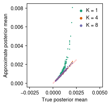
Under this model, the true posterior is
\begin{equation} \lambda_i \mid x_i, s_i \sim \Gam(a + x_i, b + s_i), \end{equation}where the true prior is \(\lambda_i \sim \Gam(a, b)\). Compare the approximate posterior mean to the true posterior mean.
cm = plt.get_cmap('Dark2')
pm = (x + np.exp(log_inv_disp)) / (s + np.exp(log_mean - log_inv_disp))
plt.clf()
plt.gcf().set_size_inches(3, 3)
plt.gca().set_aspect('equal', adjustable='datalim')
q0 = st.gamma(a=x.reshape(-1, 1) + np.exp(log_inv_disp), scale=1 / (s.reshape(-1, 1) + np.exp(log_mean - log_inv_disp)))
for i, k in enumerate(models):
  with torch.no_grad():
    samples = np.stack([models[k].qz.forward(torch.tensor(q0.rvs(), dtype=torch.float))[0].numpy() for _ in range(100)]).squeeze()
    muhat = samples.mean(axis=0)
  plt.scatter(pm, muhat, s=1, color=cm(i), label=f'K = {k}')
lim = [0, 0.0025]
plt.plot(lim, lim, lw=1, ls=':', c='r')
plt.legend(frameon=False, handletextpad=0, markerscale=4)
plt.xlabel('True posterior mean')
plt.ylabel('Approximate posterior mean')
plt.tight_layout()
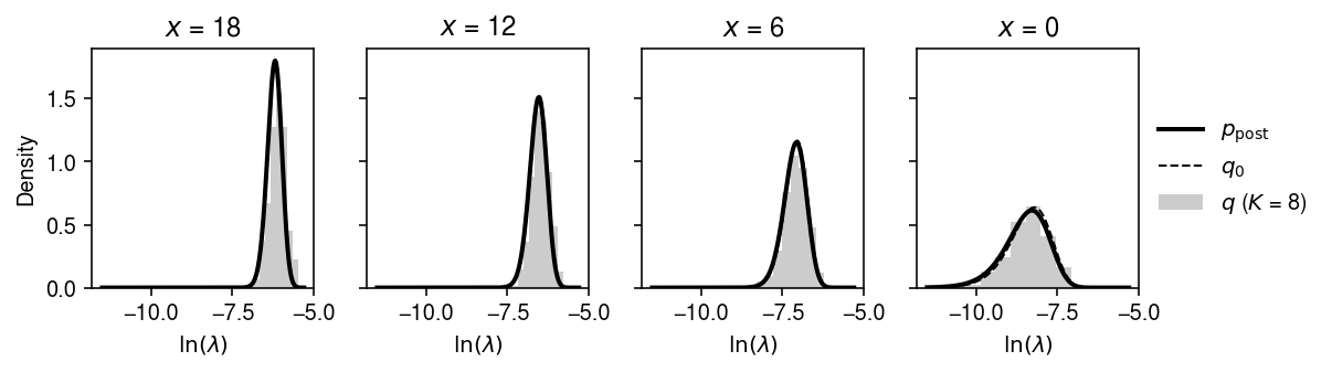
Compare the approximate posterior to the true posterior for a subset of observations.
plt.clf()
fig, ax = plt.subplots(1, 4, sharey=True)
fig.set_size_inches(8.5, 2.5)
order = np.argsort(-x)
x_grid = [18, 12, 6, 0]
for i, a in enumerate(ax):
  grid = np.log(np.linspace(1e-5, 5e-3, 1000))
  q = st.gamma(a=np.exp(fit0[1]) + x_grid[i], scale=1 / (np.exp(fit0[0] + fit0[1]) + s[0]))
  ax[i].plot(grid, q.pdf(np.exp(grid)) * np.exp(grid), lw=2, c='k', label='$p_{\mathrm{post}}$')
  q0 = st.gamma(a=x_grid[i] + np.exp(log_inv_disp), scale=1 / (s[0] + np.exp(log_mean - log_inv_disp)))
  ax[i].plot(grid, q0.pdf(np.exp(grid)) * np.exp(grid), lw=1, c='k', ls='--', label='$q_0$')
  with torch.no_grad():
    samples = models[8].qz.forward(torch.tensor(q0.rvs(size=(500, 1)), dtype=torch.float))[0].numpy()
  ax[i].hist(np.log(samples), bins=9, density=True, color='0.8', label='$q$ ($K$ = 8)')
  ax[i].set_xlabel('$\ln(\lambda)$')
  ax[i].set_title(f'$x$ = {x_grid[i]}')
ax[0].set_ylabel('Density')
ax[-1].legend(frameon=False, loc='center left', bbox_to_anchor=(1, .5))
fig.tight_layout()
Fit the model fixing \(K = 8\), comparing different initializations.
run = 11
lr = 1e-2
n_epochs = 8000
n_samples = 8
K = 8
torch.manual_seed(run)
np.random.seed(run)
models = {k: EBPM(K=K, a=a, b=b)
          .fit(torch.tensor(x.reshape(-1, 1), dtype=torch.float),
               torch.tensor(s.reshape(-1, 1), dtype=torch.float),
               n_epochs=n_epochs,
               n_samples=n_samples,
               lr=lr,
          )
          for k, a, b in zip(['Exp(1)', 'Oracle', 'Random'],
                             [1., np.exp(fit0[1]), st.expon().rvs()],
                             [1., np.exp(fit0[1] - fit0[0]), st.expon().rvs()])}
n_samples = 1000
x_grid = np.arange(x.max() + 1)
lam_grid = np.linspace(lam.min(), lam.max(), 1000)

cm = plt.get_cmap('Dark2')
plt.clf()
fig, ax = plt.subplots(2, 1)
fig.set_size_inches(4, 4)
ax[0].hist(x, bins=x_grid, density='True', color='0.7')
ax[0].plot(x_grid + 0.5, st.nbinom(n=np.exp(log_inv_disp), p=1 / (1 + s[0] * np.exp(log_mean - log_inv_disp))).pmf(x_grid), lw=2, c='k', label='Simulated')
for i, k in enumerate(models):
  F = np.array([si.simps(
    st.poisson(s * lam_grid).pmf(y) * models[k].fitted_g(torch.tensor(lam_grid.reshape(-1, 1), dtype=torch.float), log=False).ravel(),
    lam_grid)
                for y in x_grid])
  ax[0].plot(x_grid + 0.5, F, lw=1, c=cm(i), label=f'{k}')
ax[0].legend(title=f'Initialization (K = {K})', frameon=False)
ax[0].set_xticks(x_grid[::3])
ax[0].set_xlabel('Observation $x$')
ax[0].set_ylabel('Density')

ax[1].hist(lam, bins=30, density='True', color='0.7')
ax[1].plot(lam_grid, st.gamma(a=np.exp(log_inv_disp), scale=np.exp(log_mean - log_inv_disp)).pdf(lam_grid), lw=2, c='k', label='Simulated')
for i, k in enumerate(models):
  ax[1].plot(lam_grid, models[k].fitted_g(torch.tensor(lam_grid.reshape(-1, 1), dtype=torch.float), log=False), lw=1, c=cm(i), label=f'{k}')
ax[1].legend(title=f'Initialization (K = {K})', frameon=False)
ax[1].set_xlabel('Latent variable $\lambda$')
ax[1].set_ylabel('Density')

fig.tight_layout()
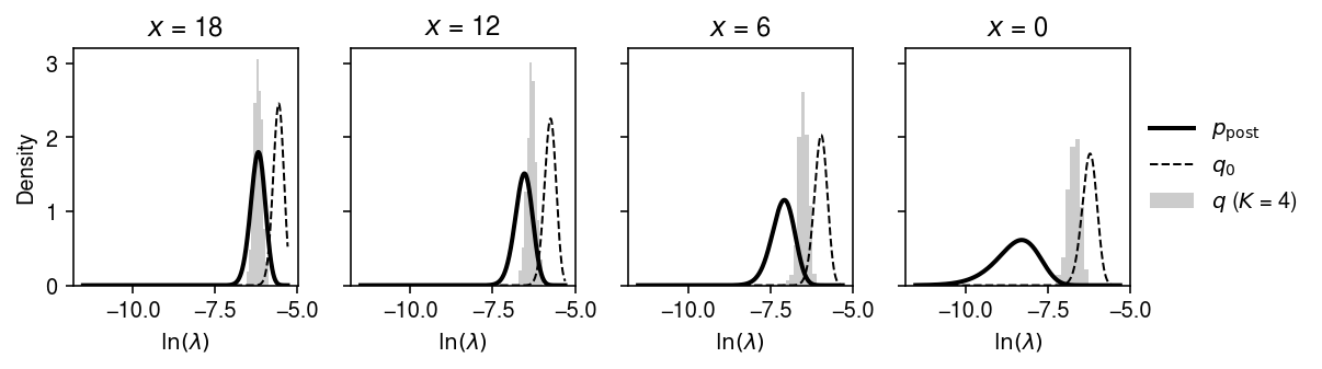
plt.clf()
fig, ax = plt.subplots(1, 4, sharey=True)
fig.set_size_inches(8.5, 2.5)
order = np.argsort(-x)
x_grid = [18, 12, 6, 0]
for i, a in enumerate(ax):
  grid = np.log(np.linspace(1e-5, 5e-3, 1000))
  q = st.gamma(a=np.exp(fit0[1]) + x_grid[i], scale=1 / (np.exp(fit0[0] + fit0[1]) + s[0]))
  ax[i].plot(grid, q.pdf(np.exp(grid)) * np.exp(grid), lw=2, c='k', label='$p_{\mathrm{post}}$')
  q0 = st.gamma(a=x_grid[i] + np.exp(3.), scale=1 / (s[0] + np.exp(fit1[0] + 3.)))
  ax[i].plot(grid, q0.pdf(np.exp(grid)) * np.exp(grid), lw=1, c='k', ls='--', label='$q_0$')
  with torch.no_grad():
    samples = models[4].qz.forward(torch.tensor(q0.rvs(size=(500, 1)), dtype=torch.float))[0].numpy()
  ax[i].hist(np.log(samples), bins=9, density=True, color='0.8', label='$q$ ($K$ = 4)')
  ax[i].set_xlabel('$\ln(\lambda)$')
  ax[i].set_title(f'$x$ = {x_grid[i]}')
ax[0].set_ylabel('Density')
ax[-1].legend(frameon=False, loc='center left', bbox_to_anchor=(1, .5))
fig.tight_layout()
EBPM example: SKP1 in iPSCs
Read the iPSC data.
dat = anndata.read_h5ad('/project2/mstephens/aksarkar/projects/singlecell-ideas/data/ipsc/ipsc.h5ad')
x = dat[:,dat.var['name'] == 'SKP1'].X.A.ravel()
z = pd.get_dummies(dat.obs['chip_id'])
s = dat.obs['mol_hs'].values.ravel()
gamma_fits = {k: scmodes.ebpm.ebpm_gamma(x[z[k].values.ravel().astype(bool)],
                                         s[z[k].values.ravel().astype(bool)],
                                         tol=1e-7)
              for k in z}
unimodal_fits = {k: scmodes.ebpm.ebpm_unimodal(x[z[k].values.ravel().astype(bool)],
                                               s[z[k].values.ravel().astype(bool)])
              for k in z}
run = 2
K = 8
n_epochs = 1500
n_samples = 1
lr = 5e-3
torch.manual_seed(run)
nf_fits = {k: EBPM(K=K, a=np.exp(gamma_fits[k][1]), b=np.exp(gamma_fits[k][1] - gamma_fits[k][0]))
               .fit(torch.tensor(x[z[k].values.ravel().astype(bool)].reshape(-1, 1), device='cuda', dtype=torch.float),
                    torch.tensor(s[z[k].values.ravel().astype(bool)].reshape(-1, 1), device='cuda', dtype=torch.float),
                    n_epochs=n_epochs,
                    n_samples=n_samples,
                    lr=lr,
                    weighted=False,
                    log_dir=f'/scratch/midway2/aksarkar/singlecell/runs/ebpm-nf-skp1-{run}-{K}-{n_samples}-{n_epochs}',
               )
           for k in ('NA18507',)}
Look at N18507.
k = 'NA18507'
idx = z[k].values.ravel().astype(bool)

x_grid = np.arange(x[idx].max() + 1)
lam_grid = np.linspace(0, (x / s).max(), 1000)

pmf = dict()
pdf = dict()
llik = dict()

pmf['Gamma'] = st.nbinom(n=np.exp(gamma_fits[k][1]), p=1 / (1 + s[idx].mean() * np.exp(gamma_fits[k][0] - gamma_fits[k][1]))).pmf(x_grid)
pdf['Gamma'] = st.gamma(a=np.exp(gamma_fits[k][1]), scale=np.exp(gamma_fits[k][0] - gamma_fits[k][1])).pdf(lam_grid)
llik['Gamma']= gamma_fits[k][-1]

g = np.array(unimodal_fits[k].rx2('fitted_g'))
a = np.fmin(g[1], g[2])
b = np.fmax(g[1], g[2])
comp_dens_conv = np.array([((st.gamma(a=k + 1, scale=1 / s.reshape(-1, 1)).cdf(b.reshape(1, -1)) - st.gamma(a=k + 1, scale=1 / s.reshape(-1, 1)).cdf(a.reshape(1, -1))) / np.outer(s, b - a)).mean(axis=0) for k in x_grid])
comp_dens_conv[:,0] = st.poisson(mu=s.reshape(-1, 1) * b[0]).pmf(x_grid).mean(axis=0)
pmf['Unimodal'] = comp_dens_conv @ g[0]
pdf['Unimodal'] = np.diff(ashr.cdf_ash(unimodal_fits[k], lam_grid).rx2('y'), prepend=0).ravel() / np.diff(lam_grid, prepend=1)
llik['Unimodal'] = np.array(unimodal_fits[k].rx2('loglik'))[0]

pdf[f'NF (K = {K})'] = np.ma.masked_invalid(nf_fits[k].fitted_g(torch.tensor(lam_grid.reshape(-1, 1), device='cuda', dtype=torch.float), log=False).ravel()).filled(0)
pmf[f'NF (K = {K})'] = np.array([si.simps(st.poisson(s.mean() * lam_grid).pmf(y) * pdf[f'NF (K = {K})'], lam_grid)
                                 for y in x_grid])
llik[f'NF (K = {K})'] = np.log(np.array([si.simps(st.poisson(sj * lam_grid).pmf(xj) * pdf[f'NF (K = {K})'], lam_grid)
                                         for xj, sj in zip(x[idx], s[idx])])).sum()
pd.Series(llik)
Gamma        -1080.578583
Unimodal     -1070.660169
NF (K = 8)   -1081.758445
dtype: float64
cm = plt.get_cmap('Dark2')

plt.clf()
fig, ax = plt.subplots(2, 1)
fig.set_size_inches(5, 4)
ax[0].hist(x[idx], bins=x_grid, color='0.7', density=True)
for i, k in enumerate(pmf):
  ax[0].plot(x_grid + 0.5, pmf[k], lw=1, c=cm(i), label=k)
ax[0].legend(frameon=False, loc='center left', bbox_to_anchor=(1, .5))
ax[0].set_xlabel('Number of molecules')
ax[0].set_ylabel('Density')
ax[0].set_title('SKP1')

ax[1].hist(x[idx] / s[idx], bins=17, color='0.7', density=True, label='$x_i / s_i$')
for i, k in enumerate(pdf):
  ax[1].plot(lam_grid, pdf[k], c=cm(i), lw=1, label=k)
ax[1].legend(frameon=False, loc='center left', bbox_to_anchor=(1, .5))
ax[1].set_xlabel('Latent gene expression')
ax[1].set_ylabel('Density')
fig.tight_layout()
EBPM real data example
Read gene expression at PPBP in PBMCs.
dat = anndata.read_h5ad('/scratch/midway2/aksarkar/modes/10k_pbmc_v3.h5ad')
x = dat[:,dat.var['name'] == 'PPBP'].X.A
s = dat.X.sum(axis=1).A
Fit Gamma and unimodal expression models.
fit0 = scmodes.ebpm.ebpm_gamma(x.ravel(), s.ravel(), tol=1e-7, extrapolate=True)
fit1 = scmodes.ebpm.ebpm_unimodal(x.ravel(), s.ravel())
0 - f5b64009-eb96-4d4a-b7d9-1c81105bf74e
run = 5
n_samples = 8
n_epochs = 1000
torch.manual_seed(run)
models = {K: EBPM(K=K,
                  a=torch.tensor(np.exp(fit0[1]), device='cuda'),
                  b=torch.tensor(np.exp(fit0[1] - fit0[0]), device='cuda'))
          .fit(torch.tensor(x, dtype=torch.float, device='cuda'),
               torch.tensor(s, dtype=torch.float, device='cuda'),
               n_samples=n_samples,
               n_epochs=n_epochs,
               lr=1e-3,
               log_dir=f'/scratch/midway2/aksarkar/singlecell/runs/ebpm-nf-ppbp-{run}-{K}-{n_samples}-{n_epochs}',
          )
          for K in (4, 8, 12)}
Plot the data and fitted models.
y = np.arange(x.max() + 1)
pmf = dict()

pmf['Gamma'] = np.array([scmodes.benchmark.gof._zig_pmf(k, size=s, log_mu=fit0[0], log_phi=-fit0[1]).mean() for k in y])

g = np.array(fit1.rx2('fitted_g'))
a = np.fmin(g[1], g[2])
b = np.fmax(g[1], g[2])
comp_dens_conv = np.array([((st.gamma(a=k + 1, scale=1 / s.reshape(-1, 1)).cdf(b.reshape(1, -1)) - st.gamma(a=k + 1, scale=1 / s.reshape(-1, 1)).cdf(a.reshape(1, -1))) / np.outer(s, b - a)).mean(axis=0) for k in y])
comp_dens_conv[:,0] = st.poisson(mu=s.reshape(-1, 1) * b[0]).pmf(y).mean(axis=0)
pmf['Unimodal'] = comp_dens_conv @ g[0]

lam_grid = np.linspace(0, (x / s).max(), 1000)[1:]
for K in models:
  pmf['K = {K}'] = [np.array([si.simps(
    st.poisson(s.mean() * lam_grid).pmf(k) * models[K].fitted_g(torch.tensor(lam_grid.reshape(-1, 1), device='cuda', dtype=torch.float), log=False).ravel(),
    lam_grid)
                              for k in y])]
0 - 5088f30c-d471-4460-8dbc-2da93b2bce98
cm = plt.get_cmap('Dark2')
plt.clf()
plt.gcf().set_size_inches(4, 2)
plt.hist(x.ravel(), bins=y, color='0.7')
for i, k in enumerate(pmf):
  plt.plot(y + 0.5, pmf[k], lw=1, c=cm(i), label=k)
plt.set_ylim(0, 10)
plt.legend(frameon=False)
plt.xlabel('Number of molecules')
plt.ylabel('Number of cells')
plt.tight_layout()
EBPM example: multi-modal prior
Draw data from a two-state kinetic model.
rng = np.random.default_rng(1)
n = 1000
s = np.full(n, 1e4)
M = 1e6
kon = 0.25
koff = 0.1
kr = 1024
p = rng.beta(a=kon, b=koff, size=n)
m = rng.poisson(kr * p)
lam = m / M
x = rng.binomial(m, s / M)
Fit the model for different choices of \(K\), initializing \(g_0\) and \(q_0\) from the Gamma component of a point-Gamma expresion model.
fit0 = scmodes.ebpm.ebpm_gamma(x, s)
fit1 = scmodes.ebpm.ebpm_point_gamma(x, s)
run = 4
lr = 1e-2
n_epochs = 24000
n_samples = 8
K = 16
torch.manual_seed(run)
models = {l: EBPM(K=K, a=a, b=b)
          .fit(torch.tensor(x.reshape(-1, 1), dtype=torch.float),
               torch.tensor(s.reshape(-1, 1), dtype=torch.float),
               n_epochs=n_epochs,
               n_samples=n_samples,
               lr=lr,
          )
          for l, a, b in zip(['Exp(1)', 'Gamma MLE', 'Point-Gamma MLE'],
                             [1., np.exp(fit0[1]), np.exp(fit1[1])],
                             [1., np.exp(fit0[1] - fit0[0]), np.exp(fit1[1] - fit1[0])])}
x_grid = np.arange(x.max() + 1)
lam_grid = np.linspace(lam.min(), 2 * lam.max(), 1000)[1:]

cm = plt.get_cmap('Dark2')
plt.clf()
fig, ax = plt.subplots(2, 1)
fig.set_size_inches(5.5, 4)
ax[0].hist(x, bins=x_grid, density='True', color='0.7')
ax[0].plot(x_grid + 0.5, st.nbinom(n=np.exp(fit0[1]), p=1 / (1 + 1e4 * np.exp(fit0[0] - fit0[1]))).pmf(x_grid), lw=1, marker='.', c=cm(5), label='Gamma')
F = st.nbinom(n=np.exp(fit1[1]), p=1 / (1 + 1e4 * np.exp(fit1[0] - fit1[1]))).pmf(x_grid)
F[1:] *= sp.expit(-fit1[2])
F[0] += sp.expit(fit1[2])
ax[0].plot(x_grid + 0.5, F, lw=1, marker='.', c=cm(6), label='Point-Gamma')
for i, k in enumerate(models):
  F = np.array([si.simps(
    st.poisson(s[0] * lam_grid).pmf(y) * models[k].fitted_g(torch.tensor(lam_grid.reshape(-1, 1), dtype=torch.float), log=False).ravel(),
    lam_grid)
                for y in x_grid])
  ax[0].plot(x_grid + 0.5, F, lw=1, c=cm(i), label=f'{k}')
ax[0].legend(title=f'Initialization (K = {K})', frameon=False, loc='center left', bbox_to_anchor=(1, .5))
ax[0].set_xticks(x_grid[::3])
ax[0].set_xlabel('Observation $x$')
ax[0].set_ylabel('Density')

ax[1].hist(lam, bins=30, density='True', color='0.7')
ax[1].plot(lam_grid, st.gamma(a=np.exp(fit0[1]), scale=np.exp(fit0[0] - fit0[1])).pdf(lam_grid), lw=1, c=cm(5), label='Gamma')
ax[1].plot(lam_grid, sp.expit(-fit1[2]) * st.gamma(a=np.exp(fit1[1]), scale=np.exp(fit1[0] - fit1[1])).pdf(lam_grid), lw=1, c=cm(6), label='Point-Gamma')
for i, k in enumerate(models):
  ax[1].plot(lam_grid, models[k].fitted_g(torch.tensor(lam_grid.reshape(-1, 1), dtype=torch.float), log=False), lw=1, c=cm(i), label=f'{k}')
ax[1].legend(title=f'Initialization (K = {K})', frameon=False, loc='center left', bbox_to_anchor=(1, .5))
ax[1].set_xlabel('Latent variable $\lambda$')
ax[1].set_ylabel('Density')

fig.tight_layout()