Dense factors

Introduction
Methods
- Idealized simulation
Results
- Idealized example

Introduction

In our simulations, fqtl fails to correctly estimate the rank of the factorization when there is a true dense tissue factor. The problem is worse in the real data application.

Methods

Idealized simulation

Simulate the easiest version of the problem.

\[ \newcommand\my{\mathbf{Y}} \newcommand\mx{\mathbf{X}} \newcommand\mi{\mathbf{I}} \newcommand\md{\mathbf{D}} \newcommand\mb{\mathbf{B}} \newcommand\vl{\mathbf{l}} \newcommand\vf{\mathbf{f}} \]

\[ \underset{n \times m}{\my} \sim \mathrm{MN}(\underset{(n \times p)}{\mx}\underset{(p \times m)}{\mb}, \underset{n \times n}{\mi}, \underset{m \times m}{\md}) \]

\[ \md = \operatorname{diag}(\sigma^2_1, \ldots, \sigma^2_m) \]

\[ \mb = \underset{(p \times 1)}{\vl} \underset{(1 \times m)}{\vf'} \]

\[ \vl_j \sim \pi_0\delta_(\cdot) + (1 - \pi_0)\mathcal{N}(0, 1) \]

\[ \vf \sim \mathcal{N}(0, \mi) \]

mnorm <- function(n, p) {
  return(matrix(rnorm(n * p), n, p))
}

sim_idealized <- function(n, p, m, pve, seed) {
  set.seed(seed)
  x <- mnorm(n, p)
  l <- rep(0, p)
  l[1] <- 1
  f <- rnorm(m)
  b <- tcrossprod(l, f)
  y <- x %*% b
  e <- sweep(mnorm(n, m), 2, sqrt((1 / pve - 1) * apply(y, 2, var)), '*')
  y <- y + e
  return(list(x=x, y=y, l=l, f=f))
}

get_fqtl_est_rank <- function(res, thresh=log(0.95 / 0.05)) {
  keep <- apply(res$mean.left$lodds > thresh, 2, any) & apply(res$mean.right$lodds > thresh, 2, any)
  return(sum(keep))
}

eval_fqtl_est_rank <- function(ntrials, k=NULL) {
  ## Important: SGVB is a stochastic algorithm, so it can get different answers
  ## even starting from a deterministic initialization.
  ##
  ## This particular simulated dataset reveals the problem we want to
  ## investigate.
  data <- sim_idealized(n=100, p=500, m=5, pve=0.5, seed=1)
  shape <- dim(data$y)
  if (is.null(k)) {
    k = min(shape[1], shape[2])
  }
  res <- lapply(1:ntrials,
         function (i) {
           res <- fqtl::fit.fqtl(
             y=scale(data$y), x.mean=scale(data$x, scale=FALSE),
             k=k, factored=TRUE,
             do.hyper=TRUE, svd.init=TRUE,
             ## Important: print.interv=1 needed for full llik trace
             vbiter=5000, verbose=FALSE, print.interv=1, rseed=i)
           list(llik=sum(res$llik[dim(res$llik)[1],]), rank=get_fqtl_est_rank(res))
         })
  return(do.call(rbind, res))
}

Results

Idealized example

Simulate a single example. Then, fit the model with \(k = 5\) (as in the benchmark). Look at different restarts from the same (deterministic) initialization.

eval_fqtl_est_rank(ntrials=3, k=5)

     llik       rank
[1,] -0.4519325 3   
[2,] -0.4532069 2   
[3,] -0.4905046 2

Now fit the model with \(k = \min(n, m)\), as in the real data analysis.

eval_fqtl_est_rank(ntrials=3)

     llik       rank
[1,] -0.4519325 3   
[2,] -0.4532069 2   
[3,] -0.4905046 2

Look at the initialization.

data <- sim_idealized(n=100, p=500, m=5, pve=0.5, seed=1)
svd(crossprod(scale(data$x, scale=FALSE), scale(data$y)) / shape[1])$d

[1] 4.115281 1.699439 1.432982 1.382543 1.359158

Idea: Should we use Tracy-Widom, sparse PCA, or even Empirical Bayes to estimate lower rank \(\mx'\my\) to use as initialization?

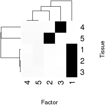
Look at the estimated factors.

res <- fqtl::fit.fqtl(
                 y=scale(data$y), x.mean=scale(data$x, scale=FALSE),
                 k=5, factored=TRUE,
                 do.hyper=TRUE, svd.init=TRUE,
                 vbiter=5000, verbose=FALSE, print.interv=1, rseed=1)

png('/project2/mstephens/aksarkar/projects/gtex_fqtl_2018/org/figure/dense.org/idealized-example-fhat.png', width=360, height=360, res=120)
par(cex.lab=2, cex.axis=2)
heatmap(res$mean.right$lodds, col=colorRampPalette(c('white', 'black'))(256), xlab='Factor', ylab='Tissue')
dev.off()